|
|
| Line 40: |
Line 40: |
| {{Bookind2}} | | {{Bookind2}} |
|
| |
|
| == Abstract==
| | {{:Store:EEMIit01}} |
|
| |
|
| An outstanding issue in cognitive neuroscience concerns how the brain is organized across different conditions. For instance, during the resting-state condition, the brain can be clustered into reliable and reproducible networks (e.g., sensory, default, executive networks). Interestingly, the same networks emerge during active conditions in response to various tasks. If similar patterns of neural activity have been found across diverse conditions, and therefore, different underlying processes and experiences of the environment, is the brain organized by a fundamental organizational principle? To test this, we applied mathematical formalisms borrowed from quantum mechanisms to model electroencephalogram (EEG) data. We uncovered a tendency for EEG signals to be localized in anterior regions of the brain during “rest”, and more uniformly distributed while engaged in a task (i.e., watching a movie). Moreover, we found analogous values to the Heisenberg uncertainty principle, suggesting a common underlying architecture of human brain activity in resting and task conditions. This underlying architecture manifests itself in the novel constant <math>K_{brain}</math>, which is extracted from the brain state with the least uncertainty. We would like to state that we are using the mathematics of quantum mechanics, but not claiming that the brain behaves as a quantum object.
| | {{:Store:EEMIit02}} |
|
| |
|
| | {{:Store:EEMIit03}} |
|
| |
|
| Subject terms: Computational science, Quantum mechanics
| | {{:Store:EEMIit04}} |
|
| |
|
| === Introduction ===
| | {{:Store:EEMIit05}} |
| An important but outstanding issue in contemporary cognitive neuroscience is understanding the organizational properties of neural activity. For instance, is there a fundamental structure to the spatial–temporal patterns neural brain activity across different conditions? One common approach used to address this question is to examine the brain at “rest”. Measures such as functional connectivity, independent component analysis and graph theoretic metrics, have been applied to data recorded using different imaging techniques (e.g., functional magnetic resonance imaging (fMRI) and electroencephalography (EEG)), to cluster brain areas that exhibit similar activity patterns. Numerous studies have shown that brain activity during “rest” can be grouped into distinct networks across<ref>Biswal, B., Zerrin Yetkin, F., Haughton, V. M. & Hyde, J. S. Functional connectivity in the motor cortex of resting human brain using echo-planar MRI. Magn. Reson. Med. 34, 537–541 (1995).</ref><ref>Hutchison,R.M.etal. Dynamic functional connectivity: Promise, issues, and interpretations. Neuroimage80,360–378(2013).</ref>; such as sensory (visual and auditory), default mode, executive, salience, and attentional (ventral and dorsal) networks that have been reliably reproduced across thousands of participants<ref>Eickhoff,S.B.,Yeo,B.T.T.&Genon,S.Imaging-basedparcellationsofthehumanbrain.Nat.Rev.Neurosci.19,672–686(2018).</ref>, and are predictive of phenotypic measures like cognition and clinical diagnoses<ref>Dajani DR, et al. Investigating functional brain network integrity using a traditional and novel categorical scheme for neurodevelopmental disorders. NeuroImage Clin. 2019;21:101678. doi: 10.1016/j.nicl.2019.101678. [PMC free article] [PubMed] [CrossRef] [Google Scholar]</ref><ref>Uddin LQ, Karlsgodt KH. Future directions for examination of brain networks in neurodevelopmental disorders. J. Clin. Child Adolesc. Psychol. 2018;47:483–497. doi: 10.1080/15374416.2018.1443461. [PMC free article] [PubMed] [CrossRef] [Google Scholar]</ref><ref>Sripada C, et al. Prediction of neurocognition in youth from resting state fMRI. Mol. Psychiatry. 2020;25:3413–3421. doi: 10.1038/s41380-019-0481-6. [PMC free article] [PubMed] [CrossRef] [Google Scholar]</ref>. These results suggest these networks may be an intrinsic aspect of neural activity.
| |
|
| |
|
| Indeed, the same set of structured patterns of neural activity have been found during "active" states, such as, while completing different tasks<ref>Biswal BB, Eldreth DA, Motes MA, Rypma B. Task-dependent individual differences in prefrontal connectivity. Cereb. Cortex. 2010;20:2188–2197. doi: 10.1093/cercor/bhp284. [PMC free article][PubMed] [CrossRef] [Google Scholar]</ref><ref>Fox MD, Raichle ME. Spontaneous fluctuations in brain activity observed with functional magnetic resonance imaging. Nat. Rev. Neurosci. 2007;8:700–711. doi: 10.1038/nrn2201. [PubMed] [CrossRef] [Google Scholar]</ref><ref>Kraus BT, et al. Network variants are similar between task and rest states. Neuroimage. 2021;229:117743. doi: 10.1016/j.neuroimage.2021.117743. [PMC free article][PubMed] [CrossRef] [Google Scholar]</ref>. For instance, there is a high degree of correspondence between networks extracted during rest and those extracted during tasks measuring sensorimotor<ref>Kristo G, et al. Task and task-free FMRI reproducibility comparison for motor network identification. Hum. Brain Mapp. 2014;35:340–352. doi: 10.1002/hbm.22180. [PMC free article][PubMed] [CrossRef] [Google Scholar]</ref><ref>Sui J, Adali T, Pearlson GD, Calhoun VD. An ICA-based method for the identification of optimal FMRI features and components using combined group-discriminative techniques. Neuroimage. 2009;46:73–86. doi: 10.1016/j.neuroimage.2009.01.026.[PMC free article] [PubMed] [CrossRef] [Google Scholar]</ref> and higher-level cognitive abilities (i.e., working memory)<ref>Calhoun VD, Kiehl KA, Pearlson GD. Modulation of temporally coherent brain networks estimated using ICA at rest and during cognitive tasks. Hum. Brain Mapp. 2008;29:828–838. doi: 10.1002/hbm.20581. [PMC free article] [PubMed] [CrossRef] [Google Scholar]</ref><ref>Xie H, et al. Whole-brain connectivity dynamics reflect both task-specific and individual-specific modulation: A multitask study. Neuroimage. 2018;180:495–504. doi: 10.1016/j.neuroimage.2017.05.050. [PMC free article] [PubMed] [CrossRef] [Google Scholar]</ref>.Even completing a task as complicated as following the plot of a movie elicits the same network architecture as observed in the resting brain<ref name=":0">Naci L, Cusack R, Anello M, Owen AM. A common neural code for similar conscious experiences in different individuals. Proc. Natl. Acad. Sci. U. S. A. 2014;111:14277–14282. doi: 10.1073/pnas.1407007111. [PMC free article] [PubMed] [CrossRef] [Google Scholar]</ref>. The correspondence between task and rest-based networks is so strong that task-based fMRI network activity can be predicted from the resting state<ref>Kannurpatti SS, Rypma B, Biswal BB. Prediction of task-related BOLD fMRI with amplitude signatures of resting-state fMRI. Front. Syst. Neurosci. 2012;6:7. doi: 10.3389/fnsys.2012.00007.[PMC free article] [PubMed] [CrossRef] [Google Scholar]</ref>, and rest-task network pairs can be identified at the individual level<ref>Elliott ML, et al. General functional connectivity: Shared features of resting-state and task fMRI drive reliable and heritable individual differences in functional brain networks. Neuroimage. 2019;189:516–532. doi: 10.1016/j.neuroimage.2019.01.068. [PMC free article][PubMed] [CrossRef] [Google Scholar]</ref>16. Together, these results suggest that rest and task-based patterns of brain activity likely share a similar underlying neural architecture, despite distinct experiences and cognitive processes<ref>Cole MW, Ito T, Cocuzza C, Sanchez-Romero R. The functional relevance of task-state functional connectivity. J. Neurosci. 2021 doi: 10.1523/JNEUROSCI.1713-20.2021. [PMC free article][PubMed] [CrossRef] [Google Scholar]</ref>.
| | {{:Store:EEMIit06}} |
|
| |
|
| There are, however, important differences between the patterns of brain activity elicited during rest and task-based paradigms, and the set of experiences and cognitive processes associated with each<ref>Zhang S, et al. Characterizing and differentiating task-based and resting state fMRI signals via two-stage sparse representations. Brain Imaging Behav. 2016;10:21–32. doi: 10.1007/s11682-015-9359-7.[PMC free article] [PubMed] [CrossRef] [Google Scholar]</ref>. For instance, the presence or absence of a task is accompanied by increases in variability across different scales including neuronal firing rates changes in field potentials<ref>Monier C, Chavane F, Baudot P, Graham LJ, Frégnac Y. Orientation and direction selectivity of synaptic inputs in visual cortical neurons: A diversity of combinations produces spike tuning. Neuron. 2003;37:663–680. doi: 10.1016/S0896-6273(03)00064-3.[PubMed] [CrossRef] [Google Scholar]</ref><ref>Churchland MM, et al. Stimulus onset quenches neural variability: A widespread cortical phenomenon. Nat. Neurosci. 2010;13:369–378. doi: 10.1038/nn.2501. [PMC free article][PubMed] [CrossRef] [Google Scholar]</ref>, variation in fMRI blood oxygen level dependent (BOLD signal)<ref name=":1">He BJ. Spontaneous and task-evoked brain activity negatively interact. J. Neurosci. 2013;33:4672–4682. doi: 10.1523/JNEUROSCI.2922-12.2013. [PMC free article][PubMed] [CrossRef] [Google Scholar]</ref> and in EEG frequency bands<ref name=":2">Bonnard M, et al. Resting state brain dynamics and its transients: A combined TMS-EEG study. Sci. Rep. 2016;6:1–9. doi: 10.1038/srep31220. [PMC free article] [PubMed] [CrossRef] [Google Scholar]</ref> Furthermore, through transcranial direct current stimulation (tDCS) it has been shown that frontal-lobe stimulation increases one’s proclivity to mind wander <ref name=":8">Axelrod V, Zhu X, Qiu J. Transcranial stimulation of the frontal lobes increases propensity of mind-wandering without changing meta-awareness. Sci. Rep. 2018;8:1–14. doi: 10.1038/s41598-018-34098-z. [PMC free article] [PubMed] [CrossRef] [Google Scholar]</ref><ref name=":3">Axelrod V, Rees G, Lavidor M, Bar M. Increasing propensity to mind-wander with transcranial direct current stimulation. Proc. Natl. Acad. Sci. U. S. A. 2015;112:3314–3319. doi: 10.1073/pnas.1421435112. [PMC free article] [PubMed] [CrossRef] [Google Scholar]</ref>. Importantly, these differences are associated with changes in properties of neural activity but not in changes in the underlying neural architecture.
| | {{:Store:EEMIit07}} |
|
| |
|
| Is there a way to identify the shared neural architecture underlying the cognitive processes associated with rest and active states while also quantifying how these processes diverge from that shared architecture of neural activity? In this paper, we applied mathematical methods analogous to those of quantum mechanics, and the concept of phase space to EEG recorded during rest and movie-watching to extract spatial and transitional properties of dynamic neural activity. Quantum mechanics was developed to describe the dynamics of the subatomic world in terms of probability amplitudes and densities of states. Quantum systems (in the Schrodinger formulation of quantum mechanics) are described by wavefunctions which square to a probability distribution leading to the loss of local determinism and the Heisenberg uncertainty principle (for an overview/intro to the subject see<ref name=":7">Townsend JS. A Modern Approach to Quantum Mechanics.University Science Books; 2012. [Google Scholar]</ref>. This uncertainty principle places a fundamental limit on the location and the momentum of a point particle <ref>Heisenberg W. Über den anschaulichen Inhalt der quantentheoretischen Kinematik und Mechanik. Z. Phys. 1927;43:172–198. doi: 10.1007/BF01397280. [CrossRef] [Google Scholar]</ref>. In essence, if the position of a particle is known there is an underlying uncertainty in its momentum (one cannot precisely say how fast it is going) and vice versa. In addition to the adaptation of the wavefunction approach to quantum mechanics in this paper, we also employed a phase space model. Phase space is a widely used tool in the study of dynamical systems, where the positional variables are paired with their conjugate momenta which establishes a multidimensional space that describes all possible configurations of the given system. This space spans the entire range of states that a system can exist in, each point (in this hyper-space) represents a single state of the system. Phase space and its assorted formalisms are a classical concept, and we simply use it as another tool for analysing the EEG data. Herein, the mathematical methods of quantum mechanics are applied to EEG data to extract a proxy to phase space. This quasi-quantum approach naturally generates the concepts of ‘average’ position, ‘average’ momentum and culminates in an analogous Heisenberg uncertainty principle.
| | {{:Store:EEMIit08}} |
|
| |
|
| In this paper, we posit that using mathematical tools drawn from quantum mechanics, an underlying pattern representative of task and resting brain activity can be realised, in which differences across conditions are apparent, but culminates in a task independent constant value. It is important to note that we are not claiming that the brain behaves as a quantum object as some believe<ref>Penrose R. The Emperor’s New Mind. Viking Penguin; 1990. [Google Scholar]</ref> <ref>Penrose R. Shadows of the Mind: A Search for the Missing Science of Consciousness. Oxford University Press; 1994. [Google Scholar]
| | {{:Store:EEMIit09}} |
|
| |
|
| </ref> <ref>Atmanspacher H. Quantum Approaches to Consciousness.Stanford Encyclopedia of Philosophy; 2004. [Google Scholar]</ref><ref>Hameroff S. How quantum brain biology can rescue conscious free will. Front. Integr. Neurosci. 2012;6:93. doi: 10.3389/fnint.2012.00093. [PMC free article] [PubMed] [CrossRef] [Google Scholar]</ref>. Rather, we have employed some of the analytical tools from the Schrodinger formulation of quantum mechanics to the brain with the aim of gaining new insight into resting and task-based brain dynamics. Not only does devising this model probe questions into the functions of the brain, but it also provides a novel approach to analysing the myriad of data available in neuroscience.
| | {{:Store:EEMIit10}} |
|
| |
|
| === Results ===
| | {{:Store:EEMIit11}} |
| In this paper, we adapted the probability amplitudes of quantum mechanics to define new metrics for examining EEG data—the ‘average position’ and ‘average momentum’ of the EEG signal. These were constructed from our definition of ‘brain states’ based on the quasi-quantum model. This allowed us to ascertain the frequency with which unique brain regions are entered by the pseudo-wavefunction, as well as explore the average-valued phase space. Finally, an analogous uncertainty relationship to that of quantum mechanics was established, with the full mathematical derivation described in the methods.
| |
|
| |
|
| ==== Average values ====
| | {{:Store:EEMIit12}} |
| The ‘average position’ of the EEG data was first extracted performing a Hilbert transform of the pre-processed time courses, and then applying a normalization constraint. Typically, the Hilbert transformed data is used to generate a metric of power dispersion or to extract the phase of the signal<ref>Freeman WJ, Vitiello G. Nonlinear brain dynamics as macroscopic manifestation of underlying many-body field dynamics. Phys. Life Rev. 2006;3:93–118. doi: 10.1016/j.plrev.2006.02.001.[CrossRef] [Google Scholar]
| |
| </ref><ref>le Van Quyen M, et al. Comparison of Hilbert transform and wavelet methods for the analysis of neuronal synchrony. J. Neurosci. Methods. 2001;111:83–98. doi: 10.1016/S0165-0270(01)00372-7.[PubMed] [CrossRef] [Google Scholar]</ref><ref>Freeman WJ. Deep analysis of perception through dynamic structures that emerge in cortical activity from self-regulated noise. Cogn. Neurodyn. 2009;3:105–116. doi: 10.1007/s11571-009-9075-3.[PMC free article] [PubMed] [CrossRef] [Google Scholar]</ref>. Instead, we imposed a new normalization condition, thereby creating an analogy to the wavefunctions of quantum mechanics. Denoting the Hilbert transformed time course of the <math>j</math>th electrode as <math>\Psi_j</math>, this is equivalent to
| |
| <center>
| |
| {| width="80%" |
| |
| |-
| |
| | width="33%" |
| |
| | width="33%" | <math>\Psi_j(t)=A_j(t)\exp (i\theta_j(t))</math>
| |
| | width="33%" align="right" | <math>(1)</math>
| |
| |}
| |
| </center>
| |
|
| |
|
| With <math>i=\sqrt{-1}</math>. We then imposed the normalization condition,
| | {{bib}} |
| <center>
| |
| {| width="80%" |
| |
| |-
| |
| | width="33%" |
| |
| | width="33%" |<math>\hat{\Psi}_j(t)= \frac{\Psi_j(t)}{\sqrt{\sum_{j=1}^{92}|\Psi_j|^2}}</math>
| |
| | width="33%" align="right" |<math>(2)</math>
| |
| |}
| |
| </center>
| |
| | |
| | |
| | |
| The summation extends to 92, corresponding to the 92 electrodes selected from the original 129 on the head cap (channels removed from the face and neck for this analysis). This normalization constraint allowed us to define the probability at time <math>t</math> of the <math>j</math> ''j''th electrode as
| |
| <center>
| |
| {| width="80%" |
| |
| |-
| |
| | width="33%" |
| |
| | width="33%" | <math>P_j(t)=\hat{\Psi}^*_j(t) \times\hat{\Psi}_j(t)</math>
| |
| | width="33%" align="right" |<math>(3)</math><br />
| |
| |}
| |
| </center>
| |
| | |
| With the * denoting complex conjugation<ref name=":7" />. We then can describe each moment in time as a ‘brain state’ that is fully described (in the context of this model) through the ‘wavefunction’. This ‘brain state’ uniquely specifies the EEG signal, and hence the dynamics of interest, at each moment in time. Using this definition of probability, we defined two average quantities of interest. The average position and momentum are given explicitly by,
| |
| | |
| <center>
| |
| {|
| |
| | width="33%" |
| |
| | width="33%" |<math>\langle x(t)\rangle=\sum_{j=1}^{92}x_jP_j(t)</math> <math>\langle p_x(t)\rangle=m{d \over dt}\langle x(t)\rangle=m\sum_{j=1}^{92}x_j{d \over dt}P_j(t)</math>
| |
| | width="33%" align="right" |<math>(4)</math>
| |
| |}
| |
| </center>
| |
| | |
| | |
| | |
| With the same holding true for y. These two equations are how we create our quasi-quantum mechanical analogues. The second equation is an extension of Ehrenfest’s theorem, relating the average momenta of a particle to the time derivative of its average position. Where we have assumed a Hamiltonian with only a spatially dependent potential. Note that as the positions are fixed in space (positions of the electrodes) only the probability changes in time. Throughout this paper the mass m has been taking to be unity for both the <math>x</math> and <math>y</math> momenta. Each of the 92 electrodes were projected onto the horizontal plane, thus the <math>j</math>th electrode was described by one unique <math>(x_j,y_j)</math> point.
| |
| | |
| We first examined this model by grouping the 92 electrodes into eight regions on the scalp: Anterior L/R, Posterior L/R, Parietal L/R, Occipital L/R and the probabilities of each electrode in the region were summed to give a region-level probability. Figure 1A shows the <math>(x_j,y_j)</math> locations of each electrode, with different colours representing each of the eight groups. Figure 1B displays the frequency of entering each region, grouped by the four task conditions and two resting conditions. This reflects the normalized count of regional probabilities integrated in time. We found that each anterior region was entered more frequently while at rest than when subjects were engaged in either movie. Specifically, the anterior left and right regions had significant within stimulus change, with <math>P<0.001</math> (Tukey adjusted) for the ''Taken Rest—Taken, Taken Rest—Taken Scrambled, BYD Rest—BYD and BYD Rest—BYD Scrambled.'' This is in line with Axelrod and colleagues’ findings which showed activation in the frontal region was associated with mind wandering<ref name=":8" /><ref name=":3" />. We found frequency suppression in posterior regions, and an increase in anterior frequency in rest compared to the stimulated conditions, consistent with fMRI studies showing increased activation in the posterior cingulate cortex, and the medial prefrontal cortex during rest <ref name=":2" /><ref name=":3" /><ref name=":4">Wang RWY, Chang WL, Chuang SW, Liu IN. Posterior cingulate cortex can be a regulatory modulator of the default mode network in task-negative state. Sci. Rep. 2019;9:1–12. [PMC free article][PubMed] [Google Scholar]</ref><ref>Uddin LQ, Kelly AMC, Biswal BB, Castellanos FX, Milham MP. Functional connectivity of default mode network components: Correlation, anticorrelation, and causality. Hum. Brain Mapp. 2009;30:625–637. doi: 10.1002/hbm.20531. [PMC free article][PubMed] [CrossRef] [Google Scholar]</ref><ref>Stawarczyk D, Majerus S, Maquet P, D’Argembeau A. Neural correlates of ongoing conscious experience: Both task-unrelatedness and stimulus-independence are related to default network activity. PLoS One. 2011;6:e16997. doi: 10.1371/journal.pone.0016997.[PMC free article] [PubMed] [CrossRef] [Google Scholar]</ref><ref name=":5">Greicius, M. D., Krasnow, B., Reiss, A. L., Menon, V. & Raichle, M. E. ''Functional Connectivity in the Resting Brain: A Network Analysis of the Default Mode Hypothesis''. www.pnas.org. [PMC free article] [PubMed]</ref>. Thus, suggesting our model captures the frontal tendency associated with the brain activity while at rest.
| |
| | |
| | |
| [[File:Figure 1.jpeg|thumb|<small>'''Figure 1:'''</small> <small>('''A''') Electrode locations for each of the 92 electrodes on the Electrical Geodesics Inc. headcap. Electrodes were projected onto a horizontal plane with the nose in the positive y direction. Electrodes have been colour-coded to display the constituent parts of the 8 groups for the frequency analysis, namely, occipital left (blue)/right (orange), parietal left (green)/right (red), posterior left (purple)/right (brown) and anterior left (pink)/right (grey). ('''B''') Histograms representing the frequency of entering each region ''fG'' are displayed for the six conditions tested. Significant within stimulus change is present between each of the Anterior Left and Right regions when comparing the pre-stimulus rest and the respective stimulated condition (''P'' < 0.001, Tukey adjusted.). Error bars display the 1 standard deviation confidence interval.</small>|alt=|center|500x500px]]
| |
| | |
| ===== Phase space =====
| |
| We also explored the average-valued phase space of this system. The phase space for each subject was plotted as the average position and momentum along the <math>x</math> direction <math>(\langle x(t)\rangle,\langle p_x(t)\rangle)</math> or as the average position and momentum along the <math>x</math> direction <math>(\langle y(t)\rangle,\langle p_y(t)\rangle)</math>. Figure 2 shows the centroids of the phase space scatter plots for each subject with an ellipse representing the one standard deviation confidence interval. Note that values are only reported for the intact stimuli as an analysis of variance shows the scrambled and intact movies are indistinguishable in phase space (P<math>P<0.85</math>, Tukey adjusted). Figure 2A and B show the projection of the phase space centroid onto the plane spanned by <math>x</math> and <math>p_x</math> for “''Bang! You’re Dead''” and “''Taken''” respectively, and Fig. 2C and D (<math>y,p_y</math>) plane. The average position along the <math>y</math> axis <math>(\langle y\rangle)</math> for the intact stimulus (“BYD” and “Taken”) and their scrambled forms are significantly different from the pre-stimulus rest counterparts with <math>P<0.001</math> (Tukey adjusted) whereas the task-positive and resting centroids are indistinguishable in the <math>x</math> plane (<math>P<0.05</math>, Tukey adjusted). The averages of the group are reported in Table Table11 along with their standard deviations. These values are the averaged value of the centroids (average of the within stimuli centre points in Fig. 2) for the respective position/momenta within each stimulus level. As also seen in Fig. 2C and D, there is a striking difference of one order of magnitude for <math>\langle y\rangle</math> between the resting and task conditions, yet no marked differences in <math>x</math>,<math>\langle p_x\rangle</math> , or <math>\langle p_y\rangle</math>.
| |
| | |
| | |
| [[File:Figure 2.jpeg|thumb|<small>'''Figure 2:''' Mean phase space centroids for each subject. Ellipses represent the 1 standard deviation confidence interval. Centroids for the scrambled stimuli were omitted as they are indistinguishable from intact stimuli (''P'' > 0.85) ('''A''') Centroids for ''“Bang! You’re Dead”'' along the x direction. ('''B''') Centroids for ''“Taken”'' along the x direction. ('''C''') Centroids for ''“Bang! You’re Dead”'' along the y direction. ('''D''') Centroids for ''“Taken”'' along the y direction. Differences are only apparent in the y direction (''P'' < 0.001, Tukey adjusted) indicative of the higher level of anterior activation as noted in Fig. 1.</small>|alt=|center|500x500px]]
| |
| | |
| | |
| | |
| | |
| === Table 1 ===
| |
| Group averages of the centroids.
| |
| | |
| {| class="wikitable"
| |
| |+
| |
| !Stimulus
| |
| !<math>\langle x\rangle</math>
| |
| !<math>\langle y\rangle</math>
| |
| !<math>\langle p_x\rangle</math>
| |
| !<math>\langle p_y\rangle</math>
| |
| |-
| |
| |Taken
| |
| | colspan="1" rowspan="1" |<small><math>(-1.4\pm5.8)\times10^{-1}</math></small>
| |
| | colspan="1" rowspan="1" |<small><math>(2.4\pm8.0)\times10^{-1}</math></small>
| |
| | colspan="1" rowspan="1" |<small><math>(-5.8\pm27.0)\times10^{-2}</math></small>
| |
| | colspan="1" rowspan="1" |<small><math>(-1.0\pm4.1)\times10^{-1}</math></small>
| |
| |-
| |
| |Taken Scrambled
| |
| | colspan="1" rowspan="1" |<small><math>(-7.7\pm35.0)\times10^{-2}</math></small>
| |
| | colspan="1" rowspan="1" |<small><math>(1.1\pm9.3)\times10^{-1}</math></small>
| |
| | colspan="1" rowspan="1" |<small><math>(4.1\pm13.0)\times10^{-2}</math></small>
| |
| | colspan="1" rowspan="1" |<small><math>(6.3\pm35.0)\times10^{-2}</math></small>
| |
| |-
| |
| | colspan="1" rowspan="1" |Bang! You’re Dead
| |
| | colspan="1" rowspan="1" |<small><math>(1.2\pm4.7)\times10^{-1}</math></small>
| |
| | colspan="1" rowspan="1" |<small><math>(3.5\pm74.0)\times10^{-2}</math></small>
| |
| | colspan="1" rowspan="1" |<small><math>(2.6\pm33.0)\times10^{-2}</math></small>
| |
| | colspan="1" rowspan="1" |<small><math>(-3.0\pm42.0)\times10^{-1}</math></small>
| |
| |-
| |
| | colspan="1" rowspan="1" |Bang! You’re Dead Scrambled
| |
| | colspan="1" rowspan="1" |<small><math>(1.4\pm5.7)\times10^{-1}</math></small>
| |
| | colspan="1" rowspan="1" |<small><math>(-2.6\pm7.5)\times10^{-1}</math></small>
| |
| | colspan="1" rowspan="1" |<small><math>(-1.5\pm2.8)\times10^{-1}</math></small>
| |
| | colspan="1" rowspan="1" |<small><math>(-5.5\pm53.0)\times10^{-2}</math></small>
| |
| |-
| |
| | colspan="1" rowspan="1" |Rest (Pre-Taken)
| |
| | colspan="1" rowspan="1" |<small><math>(-1.3\pm4.6.0)\times10^{-1}</math></small>
| |
| | colspan="1" rowspan="1" |<small><math>(2.0\pm1.4)\times10^{0}</math></small>
| |
| | colspan="1" rowspan="1" |<small><math>(9.1\pm19.0)\times10^{-2}</math></small>
| |
| | colspan="1" rowspan="1" |<small><math>(-6.3\pm7.3)\times10^{-1}</math></small>
| |
| |-
| |
| | colspan="1" rowspan="1" |Rest (Pre-BYD)
| |
| | colspan="1" rowspan="1" |<small><math>(1.1\pm66.0)\times10^{-3}</math></small>
| |
| | colspan="1" rowspan="1" |<small><math>(1.9\pm1.2)\times10^{0}</math></small>
| |
| | colspan="1" rowspan="1" |<small><math>(1.0\pm26.0)\times10^{-2}</math></small>
| |
| | colspan="1" rowspan="1" |<small><math>(-4.3\pm7.5)\times10^{-1}</math></small>
| |
| |}
| |
| | |
| | |
| Significant differences are only noted for the rest acquired before Taken and Bang! You’re Dead when comparing the average y location to either of their task counterparts (scrambled and intact stimulus).
| |
| | |
| Group averages of the centroids.
| |
| | |
| This analysis revealed two notable findings. First, there was a lack of significant differences in the momenta of the brain along the x and y direction. Second, the averages in momenta were not significantly different from 0 at the group level. The positive or negative momenta come from the competing time derivative of the probability and location of the electrode. Since the momenta average to 0, there is an equal number of anterior and posterior electrodes with both increases and decreases in probability.
| |
| | |
| Further, we examined changes in the probability values in both resting and active states. Animations of the probability distributions are present in Supplementary Material 1. In these animations, the differences in rest and task are apparent through the evolution of probability in time.
| |
| | |
| ==== Uncertainty principle ====
| |
| | |
| Despite the confirmation of previous neuroscientific results, and the apparent success of our quasi-quantum model, our research question as posed above remains only half answered. Using this model, we noted differences in the probability distributions and the phase space centroids in rest when compared to task. However, we still sought a parameter from the model that would remain the same in rest and task. To this end, we defined an analogous Heisenberg uncertainty principle of the form,
| |
| <center>
| |
| {| width="80%" |
| |
| |-
| |
| | width="33%" |
| |
| | width="33%" |<math>\bigtriangleup x(t)\bigtriangleup p_x(t)\geq K_{brain}</math>
| |
| | width="33%" align="right" |<math>(5)</math>
| |
| |}<blockquote></blockquote>
| |
| </center>
| |
| | |
| | |
| Table 2 displays the values of this constant (<math>K_{brain}</math>) acquired in all conditions, as well as the maximum value, mean value, and standard deviation. We found that this quasi-quantum model leads to a constant minimum value across <math>\Delta x(t)\Delta p_x(t)</math> and <math>\Delta y(t)\Delta p_y(t)</math> of <math>0,78\pm0,41\tfrac{cm^2}{4ms}</math> with <math>T=0, P=1</math>. Note the unit of <math>\tfrac{cm^2}{4ms}</math> is a result of the EEG being sampled at 250 Hz and the mass being taken to be unity. Furthermore, the average value and standard deviation of these quantities remains consistent across conditions with an average value of <math>9,3\pm4,4\tfrac{cm^2}{4ms}</math> (<math>T=0, P=1</math>) and a standard deviation of <math>18\pm29\tfrac{cm^2}{4ms}</math> (<math>T=0, P=1</math>).
| |
| Notably, the maximum value does vary between conditions, with the largest value occurring while subjects watched the intact clip from Bang! You’re Dead. Despite the average position of the signal along the y direction being different in rest than during a task (<math>P<0.001</math>), the quasi-quantum mathematical methodology leads to a constant uncertainty value. Quite remarkably, the values in the table display that the average uncertainty and minimum uncertainty is the same across different conditions, despite maxima varying by over two orders of magnitude. Thus, giving further credence to the idea that this uncertainty relation captures the similarities of the brain across the vastly different conditions. Figure 3 displays the probability distribution at the time corresponding to the minimum in uncertainty for both <math>x</math> and <math>y</math>.
| |
| | |
| | |
| === Table 2===
| |
| | |
| {| class="wikitable"
| |
| !Stimulus
| |
| !<math>\Delta x\Delta p_x</math>
| |
| !<math>\Delta y\Delta p_y</math>
| |
| !<math>\Delta x\Delta p_x</math>
| |
| !<math>\Delta y\Delta p_y</math>
| |
| !<math>\Delta x\Delta p_x</math>
| |
| !<math>\Delta y\Delta p_y</math>
| |
| !<math>\Delta x\Delta p_x</math>
| |
| !<math>\Delta y\Delta p_y</math>
| |
| |-
| |
| | colspan="1" rowspan="1" |Taken
| |
| | colspan="1" rowspan="1" |<small><math display="inline">(7\pm2.1)10^{-1}</math></small>
| |
| | colspan="1" rowspan="1" |<small><math display="inline">(7.2\pm1.8)10^{-1}</math></small>
| |
| | colspan="1" rowspan="1" |<small><math display="inline">(1.9\pm1.0)10^{3}</math></small>
| |
| | colspan="1" rowspan="1" |<small><math display="inline">(1.4\pm0.8)10^{3}</math></small>
| |
| | colspan="1" rowspan="1" |<small><math display="inline">(8.2\pm2.2)10^{0}</math></small>
| |
| | colspan="1" rowspan="1" |<small><math display="inline">(8.2\pm2.2)10^{0}</math></small>
| |
| | colspan="1" rowspan="1" |<small><math display="inline">(1.4\pm0.4)10^{1}</math></small>
| |
| | colspan="1" rowspan="1" |<small><math display="inline">(1.3\pm0.4)10^{1}</math></small>
| |
| |-
| |
| | colspan="1" rowspan="1" |Taken Scrambled
| |
| | colspan="1" rowspan="1" |<small><math display="inline">(6.4\pm2.6)10^{-1}</math></small>
| |
| | colspan="1" rowspan="1" |<small><math display="inline">(6.8\pm2.1)10^{-1}</math></small>
| |
| | colspan="1" rowspan="1" |<small><math display="inline">(1.7\pm1.2)10^{3}</math></small>
| |
| | colspan="1" rowspan="1" |<small><math display="inline">(2.1\pm2.2)10^{3}</math></small>
| |
| | colspan="1" rowspan="1" |<small><math display="inline">(8.1\pm1.9)10^{0}</math></small>
| |
| | colspan="1" rowspan="1" |<small><math display="inline">(7.8\pm2.0)10^{0}</math></small>
| |
| | colspan="1" rowspan="1" |<small><math display="inline">(1.4\pm0.4)10^{1}</math></small>
| |
| | colspan="1" rowspan="1" |<small><math display="inline">(1.4\pm0.7)10^{1}</math></small>
| |
| |-
| |
| | colspan="1" rowspan="1" |Bang! You’re Dead
| |
| | colspan="1" rowspan="1" |<small><math display="inline">(7.6\pm4.9)10^{-1}</math></small>
| |
| | colspan="1" rowspan="1" |<small><math display="inline">(7.5\pm3.1)10^{-1}</math></small>
| |
| | colspan="1" rowspan="1" |<small><math display="inline">(0.1\pm3.1)10^{5}</math></small>
| |
| | colspan="1" rowspan="1" |<small><math display="inline">(0.7\pm1.4)10^{4}</math></small>
| |
| | colspan="1" rowspan="1" |<small><math display="inline">(9.4\pm6.7)10^{0}</math></small>
| |
| | colspan="1" rowspan="1" |<small><math display="inline">(8.3\pm3.6)10^{0}</math></small>
| |
| | colspan="1" rowspan="1" |<small><math display="inline">(4.1\pm8.9)10^{1}</math></small>
| |
| | colspan="1" rowspan="1" |<small><math display="inline">(2.7\pm3.9)10^{1}</math></small>
| |
| |-
| |
| |colspan="1" rowspan="1" |Bang! You’re Dead Scrambled
| |
| | colspan="1" rowspan="1" |<small><math display="inline">(7.4\pm3.2)10^{-1}</math></small>
| |
| | colspan="1" rowspan="1" |<small><math display="inline">(7.1\pm2.9)10^{-1}</math></small>
| |
| | colspan="1" rowspan="1" |<small><math display="inline">(2.5\pm1.2)10^{3}</math></small>
| |
| | colspan="1" rowspan="1" |<small><math display="inline">(2.5\pm1.6)10^{3}</math></small>
| |
| | colspan="1" rowspan="1" |<small><math display="inline">(9.3\pm5.1)10^{0}</math></small>
| |
| | colspan="1" rowspan="1" |<small><math display="inline">(8.6\pm4.4)10^{0}</math></small>
| |
| | colspan="1" rowspan="1" |<small><math display="inline">(1.6\pm0.7)10^{1}</math></small>
| |
| | colspan="1" rowspan="1" |<small><math display="inline">(1.5\pm0.8)10^{1}</math></small>
| |
| |-
| |
| |colspan="1" rowspan="1" |Rest (Pre-Taken)
| |
| | colspan="1" rowspan="1" |<small><math display="inline">(9.7\pm4.2)10^{-1}</math></small>
| |
| | colspan="1" rowspan="1" |<small><math display="inline">(1.1\pm0.6)10^{0}</math></small>
| |
| | colspan="1" rowspan="1" |<small><math display="inline">(3.5\pm3.1)10^{2}</math></small>
| |
| | colspan="1" rowspan="1" |<small><math display="inline">(3.5\pm1.7)10^{2}</math></small>
| |
| | colspan="1" rowspan="1" |<small><math display="inline">(9.6\pm2.1)10^{0}</math></small>
| |
| | colspan="1" rowspan="1" |<small><math display="inline">(1.3\pm0.4)10^{1}</math></small>
| |
| | colspan="1" rowspan="1" |<small><math display="inline">(1.5\pm0.8)10^{1}</math></small>
| |
| | colspan="1" rowspan="1" |<small><math display="inline">(1.9\pm0.7)10^{1}</math></small>
| |
| |-
| |
| |Rest (Pre-BYD)
| |
| | colspan="1" rowspan="1" |<small><math display="inline">(6.3\pm3.7)10^{-1}</math></small>
| |
| | colspan="1" rowspan="1" |<small><math display="inline">(8.6\pm6.1)10^{-1}</math></small>
| |
| | colspan="1" rowspan="1" |<small><math display="inline">(3.7\pm2.0)10^{2}</math></small>
| |
| | colspan="1" rowspan="1" |<small><math display="inline">(4.3\pm2.5)10^{2}</math></small>
| |
| | colspan="1" rowspan="1" |<small><math display="inline">(8.7\pm3.3)10^{0}</math></small>
| |
| | colspan="1" rowspan="1" |<small><math display="inline">(1.2\pm0.6)10^{1}</math></small>
| |
| | colspan="1" rowspan="1" |<small><math display="inline">(1.4\pm0.5)10^{1}</math></small>
| |
| | colspan="1" rowspan="1" |<small><math display="inline">(1.9\pm0.8)10^{1}</math></small>
| |
| |}
| |
| Various values extracted from the time courses of the products
| |
| <math>\Delta x(t)\Delta p_x(t)</math> and <math>\Delta y(t)\Delta p_y(t)</math>.
| |
| | |
| | |
| | |
| [[File:Figure 3.jpeg|center|thumb|788x788px|<small>'''Figura 3:''' Probability maps corresponding to the least uncertain time point for each of the six experimental conditions. ('''A''') The probabilities which lead to the minimum uncertainty as defined by the minimum of . ('''B''') The probabilities which lead to the minimum uncertainty as defined by the minimum of . One subject is displayed for all Taken stimuli, and another for all Bang! You’re Dead stimuli.</small>]]
| |
| | |
| | |
| | |
| ==== Discussion ====
| |
| | |
| In the current study, we investigated the spatial-extent and the associated transitional properties of neural activity in the brain during active and resting conditions, and whether similar underlying network properties exist. We found that applying the Hilbert transformation to the EEG data and normalizing it (Eq. 2) imposes a probabilistic structure to the EEG signal across the brain (Eq. 3), which we used to identify probability of spatial patterns of activity along with transitions in activity across the scalp. We found more anterior activity during rest relative to the movie watching, in both amplitude and phase space. This finding is in line with previous results showing increased activation in anterior region during rest <ref name=":1" /><ref name=":1" /><ref name=":2" /><ref name=":4" /><ref name=":5" /><ref>Christoff K, Gordon AM, Smallwood J, Smith R, Schooler JW. Experience sampling during fMRI reveals default network and executive system contributions to mind wandering. Proc. Natl. Acad. Sci. U. S. A. 2009;106:8719–8724. doi: 10.1073/pnas.0900234106.[PMC free article] [PubMed] [CrossRef] [Google Scholar]</ref>. Moreover, by normalizing the Hilbert transformed EEG signals and extracting average values akin to those of the wavefunction formulation of quantum mechanics, we were able to compute uncertainty in the ‘position’ and ‘momentum’ during rest and movie-watching, which is set by the new constant
| |
| <math>K_{brain}=0,78\pm0,41\tfrac{cm^2}{4ms}</math>.
| |
| | |
| It is alluring to associate the constant related to the ‘position’ and ‘momentum’ of neural activity to a fundamental principle, such as, the Heisenberg uncertainty principle. However, it is still unclear what this uncertainty means. It could imply limits to the degree to which the brain is accessible; increasing information about the precise location of the brain state (as described by our quasi-quantum ‘wavefunctions’) will produce a bigger uncertainty about where it will be at a subsequent time. These results offer an interesting perspective on the link between neural function and cognitive processes. For instance, as the ‘wavefunction’ becomes localized in space along a train of thoughts, we become distracted to increase the uncertainty, which may explain why minds wander and thoughts are fleeting?
| |
| | |
| Is the <math> K_b </math> value we found constant across different stimulus conditions, and independent of the number of electrodes used to acquire the data? To test this, we down sampled the EEG electrodes from 92 to 20 and performed the same analysis as in the main text. In line with 92 channels, we found the anterior tendency in rest, but we found reducing the electrodes to 20 resulted in a different constant <math>K_b= 0,03\pm0,02\tfrac{cm^2}{4ms}</math> (See Supplementary Material). This demonstrates that the model is able to capture the differences of rest/task, but a montage-dependent normalisation condition may need to be introduced.
| |
| | |
| It is important to note that uncertainty values of this form are inherent to any Fourier conjugate variables, as a value spreads out in one variable, it localizes in the other. This suggests that after defining the square of the Hilbert transformed EEG electrode time course to be the probability and imposing the properties of a Hilbert space onto the electrode signals, an uncertainty values can be extracted. In quantum mechanics, this uncertainty sets the limit for the scales that cannot be observed. This approach was inspired from the need in neuroscience for novel models to help interpret neuroimaging data. While this is an interesting methodological step forward, we still must determine if the observed uncertainty in the EEG data is supported by a new fundamental principle like in quantum mechanics, or if it is just the outcome of having built two new Fourier conjugate variables from the EEG signal.
| |
| | |
| Further work must be done to explore this constant with respect to the rich taxonomy of tasks and stimuli and varying states of consciousness that are routinely used in cognitive neuroscience. This methodology could be extended into fMRI, where the BOLD time courses could be Hilbert transformed creating a three-dimensional analogue of the EEG model presented in this paper.
| |
| | |
| Ultimately, this paper presented a novel methodology for analysing EEG data. Normalizing the data and treating it as a probability amplitude led to parameters that changed with the presence or lack of stimulus, while simultaneously establishing a constant value independent of stimulus. We have successfully applied a mathematical framework based on the formalisms of quantum mechanics to the resting and task paradigm in EEG (without claiming the brain is a quantum object). As neuroscience continues to evolve, the analytic tools at its disposal must also progress accordingly. We hope that this analytical tool, along with the advances in modelling and machine learning will aid in our understanding of the nature of consciousness.
| |
| | |
| == Methods==
| |
| | |
| === Data acquisition===
| |
| Twenty-eight healthy subjects were recruited from The Brain and Mind Institute at the University of Western Ontario, Canada to participate in this study. Informed written consent was acquired prior to testing from all participants. Ethics approval for this study was granted by the Health Sciences Research Ethics Board and the Non-Medical Research Ethics Board of The University of Western Ontario and all research was performed in accordance with the relevant guidelines/regulations and in accordance with the Declaration of Helsinki.
| |
| | |
| Two suspenseful movie clips were used as the naturalistic stimuli in this study. A video clip from the silent film “Bang! You’re Dead” and an audio excerpt from the movie “Taken” were shown to 13 and 15 subjects respectively in both their original intact and scrambled forms. Prior to the two acquisitions, a section of rest was acquired where the subjects were asked to relax, without any overt stimulation. Stimulus presentation was controlled with the Psychtoolbox plugin for MATLAB <ref>Brainard DH. The psychophysics toolbox. Spat. Vis. 1997;10:433–436. doi: 10.1163/156856897X00357. [PubMed] [CrossRef] [Google Scholar]</ref><ref>Kleiner M, et al. What’s new in psychtoolbox-3. Perception. 2007;36:1–16. [Google Scholar]</ref><ref>Pelli DG. The VideoToolbox software for visual psychophysics: Transforming numbers into movies. Spat. Vis. 1997;10:437–442. doi: 10.1163/156856897X00366. [PubMed] [CrossRef] [Google Scholar]</ref> on a 15″ Apple MacBook Pro. Audio were presented binaurally at a comfortable listening volume through Etymotics ER-1 headphones.
| |
| | |
| EEG data were collected using a 129-channel cap (Electrical Geodesics Inc. [EGI], Oregon, USA). Electrode impedances were kept below 50 kΩ with signals sampled at 250 Hz and referenced to the central vertex (Cz). Using the EEGLAB MATLAB toolbox<ref>Makeig, S. & Onton, J. ERP features and EEG dynamics: An ICA perspective. In ''The Oxford Handbook of Event-Related Potential Components'' (Oxford University Press, 2012). 10.1093/oxfordhb/9780195374148.013.0035.</ref>, noisy channels were identified and removed, then interpolated back into the data. A Kolmogorov–Smirnov (KS) test on the data was used to identify regions that were not Gaussian. Independent components analysis (ICA) was then used to visually identify patterns of neural activity characteristic of eye and muscle movements which were subsequently removed from the data. EEG pre-processing was performed individually for each subject and condition.
| |
| | |
| Of the two movie clips tested, the first was an 8-min segment from Alfred Hitchcock’s TV silent movie “Bang! You’re Dead”. This scene portrays a 5-year-old boy who picks up his uncle’s revolver. The boy loads a bullet into the gun and plays with it as if it were a toy. The boy (and viewer) rarely knows whether the gun has a bullet in its chamber and suspense builds as the boy spins the chamber, points it at others, and pulls the trigger. As an alternative to visual stimulation, a 5-min audio excerpt from the movie “Taken” was also used. This clip portrays a phone conversation in which a father overhears his daughters’ kidnapping.
| |
| | |
| Furthermore, two “scrambled” control stimuli were used—one for each movie. This separates the neural responses elicited by the sensory properties of watching or listening to the movies from those involved in following the plot. The scrambled version of “Bang! You’re Dead” was generated by isolating 1 s segments and pseudorandomly shuffling the segments, thereby eliminating the temporal coherence of the narrative<ref name=":0" /> <ref name=":6">Laforge G, Gonzalez-Lara LE, Owen AM, Stojanoski B. Individualized assessment of residual cognition in patients with disorders of consciousness. NeuroImage Clin. 2020;28:102472. doi: 10.1016/j.nicl.2020.102472. [PMC free article] [PubMed] [CrossRef] [Google Scholar]</ref>. The scrambled version of “Taken” was created by spectrally rotating the audio, thus rendering the speech indecipherable<ref name=":6" /><ref>Naci L, Sinai L, Owen AM. Detecting and interpreting conscious experiences in behaviorally non-responsive patients. Neuroimage. 2017;145:304–313. doi: 10.1016/j.neuroimage.2015.11.059.[PubMed] [CrossRef] [Google Scholar]</ref>. The scrambled movie clips were presented before the intact versions to prevent potential carry-over effects of the narrative. Prior to subjects watching/listening to the scrambled stimulus a short segment of resting EEG was acquired.
| |
| | |
| == Model ==
| |
| | |
| Each of the j electrodes is described by an ordered pair (<math>x_j,y_j,z_j</math>) in 3-dimensional space. To complete this analysis, the electrodes were first projected onto the (<math>x,y</math>) plane, removing the depth of the head. Figure 1A shows the locations of each electrode in this 2d-space. Following this projection, the time courses for each of the 92 electrodes were Hilbert transformed and then normalized following the procedure listed using Eq. (2). A probability was defined in this electrode-position space as the square of the Hilbert transformed time course (Eq. 3), analogous to the wavefunctions of quantum mechanics. Eight regions Anterior L/R, Posterior L/R, Parietal L/R, Occipital L/R) were then defined by grouping the 92 electrodes, and the frequencies of entering each region fG were obtained by summing the probabilities electrodes within the group, then integrating in time.
| |
| | |
| <center>
| |
| {| width="80%" |
| |
| |-
| |
| | width="33%" |
| |
| | width="33%" |<math>Prob_G(t)=\sum_{j=1}^{92} \Psi_k^* (t)\times\Psi_k (t); f_G=\tfrac{1}{T}\sum_{j=1}^{T}Prob_G(t)</math>
| |
| | width="33%" align="right" |<math>(6)</math>
| |
| |}
| |
| </center>
| |
| | |
| where each of the eight groups denoted by the subscript have a different number of constituent electrodes N. In the occipital left and right there are 10 electrodes each, in the parietal left and right there are 17 electrodes each, in the posterior left and right there are 10 and 11 electrodes respectively, and in the anterior left and right there are 8 and 9 electrodes respectively.
| |
| | |
| Upon getting the group level frequencies average values for position and momentum were calculated using Eqs. (4) and (5) (with identical expressions for y). Finally, to ascertain our analogous uncertainty principle, we sought expressions of the form
| |
| | |
| <center>
| |
| {| width="80%" |
| |
| |-
| |
| | width="33%" |
| |
| | width="33%" |<math>\bigtriangleup x=\sqrt{\langle x^2(t)\rangle-\langle x(t)\rangle^2};
| |
| \bigtriangleup p_x=\sqrt{\langle p_x^2(t)\rangle-\langle p_x(t)\rangle^2}</math>
| |
| | width="33%" align="right" |<math>(7)</math>
| |
| |}
| |
| </center>
| |
| | |
| | |
| The expression for can be readily applied to the probabilities and positions as defined above, resulting in the first term given by
| |
| <center>
| |
| {| width="80%" |
| |
| |-
| |
| | width="33%" |
| |
| | width="33%" |<math>\langle x^2(t)\rangle=\sum_{j=1}^{92}P_j(t) x_j^2</math>
| |
| | width="33%" align="right" |<math>(8)</math>
| |
| |}
| |
| </center>
| |
| | |
| And the second term given by the square of Eq. (4). The second term of <math>\Delta P_x</math> is given by the square of Eq. (5), but the first term is more nuanced. This is owing to the complex number returned when acting the derivative operator twice on the probability. To overcome this, Fourier transforms were used to change Eq. (5) into the momentum basis which then allowed for the efficient calculation of <math>P_x^2(t)</math>.
| |
| | |
| Denoting <math>\tilde{P}_j(t)</math> as the momentum-space probability obtained through a 2-dimensional, non-uniform Fourier transform of the position space pseudo-wavefunction, Eq. (5) can be rewritten as,
| |
| | |
| <center>
| |
| {| width="80%" |
| |
| |-
| |
| | width="33%" |
| |
| | width="33%" |<math>\langle p_x(t)\rangle=\sum_{j=1}^{92}\tilde{P}_j(t)p_j</math>
| |
| | width="33%" align="right" |<math>(9)</math>
| |
| |}
| |
| </center>
| |
| Leading to the first term in the expression to be written as,
| |
| | |
| <center>
| |
| {| width="80%" |
| |
| |-
| |
| | width="33%" |
| |
| | width="33%" |<math>\langle p_x^2(t)\rangle=m^2\sum_{j=1}^{92}\tfrac{x_j^2}{\tilde{p}_j(t)}[{d \over dt}P_j(t)]^2</math>
| |
| | width="33%" align="right" |<math>(10)</math>
| |
| |}
| |
| </center>
| |
| | |
| The FINUFFT python wrapper was used to take the Fourier transform using a type 3, 2d non-uniform FFT<ref>Barnett AH, Magland J, Klinteberg LAF. A parallel nonuniform fast Fourier transform library based on an “Exponential of semicircle” kernel. SIAM J. Sci. Comput. 2019;41:C479–C504. doi: 10.1137/18M120885X. [CrossRef] [Google Scholar]</ref><ref>Barnett, A. H. Aliasing error of the kernel in the nonuniform fast Fourier transform. arXiv:2001.09405 [math.NA] (2020).</ref>, and the minimum value in time of the uncertainty relation was found. Points in momentum space were sampled on <math>p_x\in[-4,4]</math> and <math>p_y\in[-4,5]</math> along with the two additional points (<math>[-5,-4]</math>) and (<math>[-4,-5]</math>).
| |
| | |
| Figure 4 shows the position and momentum probabilities respectively in their own basis. An animation showing how these evolve in time for the different conditions is presented in Supplementary Material 2.
| |
| | |
| | |
| [[File:Figure 4.jpeg|center|thumb|500x500px|<small>'''Figure 4: (A''') Probability distribution for a single subject in the position basis. ('''B''') Momentum basis probability distribution for a single subject. The momentum values used for the Fourier transform are indicated by the point locations. Points are colour-/size-coded to represent the probability value at that location.</small>]]
| |
| | |
| To compute the values reported in Table 2, the corresponding value was found for each subject, and these were used to calculate the group average reported here.
| |
| | |
| == Supplementary Information ==
| |
| | |
| Supplementary Figures.(28M, docx)
| |
| | |
| Supplementary Information.(375K, docx)
| |
| | |
| == Acknowledgements==
| |
| We would like to thank Silvano Petrarca for his continued assistance in devising the model. This study was funded by the NSERC Discovery Grant (05578–2014RGPIN), CERC (215063), CIHR Foundation Fund (167264). AMO is a Fellow of the CIFAR Brain, Mind, and Consciousness Program.
| |
| | |
| == Author contributions==
| |
| | |
| N.J.M.P., C.M. and G.L. performed the analysis. A.S., B.S. and N.J.M.P. developed the model. A.S. and B.S. supervised the analysis. N.J.M.P., A.S., G.L. and B.S. wrote the manuscript. A.M.O. revised the manuscript.
| |
| | |
| == Competing interests ==
| |
| | |
| The authors declare no competing interests.
| |
| | |
| == Footnotes==
| |
| | |
| === Publisher's note===
| |
| | |
| Springer Nature remains neutral with regard to jurisdictional claims in published maps and institutional affiliations.
| |
|
| |
|
| These authors contributed equally: Bobby Stojanoski and Andrea Soddu.
| | {{apm}} |
| | |
| === Supplementary Information===
| |
| | |
| The online version contains supplementary material available at 10.1038/s41598-021-97960-7.
| |
| | |
| == Article information==
| |
| Sci Rep. 2021; 11: 19771.
| |
| | |
| Published online 2021 Oct 5. doi: 10.1038/s41598-021-97960-7
| |
| | |
| PMCID: PMC8492705
| |
| | |
| PMID: 34611185
| |
| | |
| Nicholas J. M. Popiel,<sup>1,2</sup> Colin Metrow,<sup>1</sup> Geoffrey Laforge,<sup>3</sup> Adrian M. Owen,<sup>3,4,5</sup> Bobby Stojanoski,<sup>#4,6</sup> and Andrea Soddu<sup>#1,3</sup>
| |
| | |
| <sup>1</sup>The Department of Physics and Astronomy, The University of Western Ontario, London, ON N6A 5B7 Canada
| |
| | |
| <sup>2</sup>Cavendish Laboratory, University of Cambridge, Cambridge, CB3 0HE UK
| |
| | |
| <sup>3</sup>The Brain and Mind Institute, The University of Western Ontario, London, ON N6A 5B7 Canada
| |
| | |
| <sup>4</sup>The Department of Psychology, The University of Western Ontario, London, ON N6A 5B7 Canada
| |
| | |
| <sup>5</sup>The Department of Physiology and Pharmacology, The University of Western Ontario, London, ON N6A 5B7 Canada
| |
| | |
| <sup>6</sup>Faculty of Social Science and Humanities, University of Ontario Institute of Technology, 2000 Simcoe Street North, Oshawa, ON L1H 7K4 Canada
| |
| | |
| Andrea Soddu, Email: asoddu@uwo.ca
| |
| | |
| Corresponding author.
| |
| | |
| #Contributed equally.
| |
| | |
| Received 2021 Apr 28; Accepted 2021 Aug 30.
| |
| | |
| Copyright © The Author(s) 2021
| |
| | |
| === Open Access ===
| |
| This article is licensed under a Creative Commons Attribution 4.0 International License, which permits use, sharing, adaptation, distribution and reproduction in any medium or format, as long as you give appropriate credit to the original author(s) and the source, provide a link to the Creative Commons licence, and indicate if changes were made. The images or other third party material in this article are included in the article's Creative Commons licence, unless indicated otherwise in a credit line to the material. If material is not included in the article's Creative Commons licence and your intended use is not permitted by statutory regulation or exceeds the permitted use, you will need to obtain permission directly from the copyright holder. To view a copy of this licence, visit http://creativecommons.org/licenses/by/4.0/.
| |
| | |
| Articles from Scientific Reports are provided here courtesy of == Nature Publishing Group ==
| |
| | |
| {{bib}} | |
Free resource
| Title
|
Esplorare l'elettroencefalografia con un modello ispirato alla meccanica quantistica
|
| Authors
|
Nicholas J. M. Popiel · Colin Metrow · Geofrey Laforge · Adrian M. Owen · Bobby Stojanoski · Andrea Soddu
|
| Source
|
Document
|
| Date
|
2021
|
| Journal
|
Sci Rep
|
| DOI
|
10.1038/s41598-021-97960-7
|
| PUBMED
|
https://pubmed.ncbi.nlm.nih.gov/34611185
|
| PDF copy
|
|
| License
|
CC BY
|
| This resource has been identified as a Free Scientific Resource, this is why Masticationpedia presents it here as a mean of gratitude toward the Authors, with appreciation for their choice of releasing it open to anyone's access
|
This is free scientific content. It has been released with a free license, this is why we can present it here now, for your convenience. Free knowledge, free access to scientific knowledge is a right of yours; it helps Science to grow, it helps you to have access to Science
This content was relased with a 'CC BY' license.
You might perhaps wish to thank the Author/s
Exploring electroencephalography with a model inspired by quantum mechanics
|
|
Free resource by Nicholas J. M. Popiel · Colin Metrow · Geofrey Laforge · Adrian M. Owen · Bobby Stojanoski · Andrea Soddu
|
Nicholas J. M. Popiel,1,2 Colin Metrow,1 Geoffrey Laforge,3 Adrian M. Owen,3,4,5 Bobby Stojanoski,#4,6 and Andrea Soddu#1,3
1The Department of Physics and Astronomy, The University of Western Ontario, London, ON N6A 5B7 Canada
2Cavendish Laboratory, University of Cambridge, Cambridge, CB3 0HE UK
3The Brain and Mind Institute, The University of Western Ontario, London, ON N6A 5B7 Canada
4The Department of Psychology, The University of Western Ontario, London, ON N6A 5B7 Canada
5The Department of Physiology and Pharmacology, The University of Western Ontario, London, ON N6A 5B7 Canada
6Faculty of Social Science and Humanities, University of Ontario Institute of Technology, 2000 Simcoe Street North, Oshawa, ON L1H 7K4 Canada
Abstract
Una questione in sospeso nelle neuroscienze cognitive riguarda il modo in cui il cervello è organizzato in diverse condizioni. Ad esempio, durante la condizione di riposo, il cervello può essere raggruppato in reti affidabili e riproducibili (ad esempio, reti sensoriali, predefinite, esecutive). È interessante notare che le stesse reti emergono durante condizioni attive in risposta a vari compiti. Se modelli simili di attività neurale sono stati trovati in condizioni diverse e, quindi, diversi processi ed esperienze sottostanti dell'ambiente, il cervello è organizzato da un principio organizzativo fondamentale? Per verificarlo, abbiamo applicato formalismi matematici presi in prestito dai meccanismi quantistici per modellare i dati dell'elettroencefalogramma (EEG). Abbiamo scoperto una tendenza per i segnali EEG a essere localizzati nelle regioni anteriori del cervello durante il "riposo" e distribuiti in modo più uniforme mentre sono impegnati in un'attività (cioè, guardando un film). Inoltre, abbiamo trovato valori analoghi al principio di indeterminazione di Heisenberg, suggerendo un'architettura sottostante comune dell'attività cerebrale umana in condizioni di riposo e di attività. Questa architettura sottostante si manifesta nella nuova costante  , che viene estratto dallo stato cerebrale con la minima incertezza. Vorremmo affermare che stiamo usando la matematica della meccanica quantistica, ma non pretendiamo che il cervello si comporti come un oggetto quantistico.
Introduzione
Una questione importante ma eccezionale nella neuroscienza cognitiva contemporanea è la comprensione delle proprietà organizzative dell'attività neurale. Ad esempio, esiste una struttura fondamentale per i modelli spazio-temporali dell'attività cerebrale neurale in condizioni diverse? Un approccio comune utilizzato per rispondere a questa domanda è quello di esaminare il cervello a "riposo". Misure come la connettività funzionale, l'analisi dei componenti indipendenti e le metriche teoriche dei grafici sono state applicate ai dati registrati utilizzando diverse tecniroche di imaging (ad esempio, risonanza magnetica funzionale (fMRI) ed elettroencefalografia (EEG)), per raggruppare aree cerebrali che mostrano schemi di attività simili . Numerosi studi hanno dimostrato che l'attività cerebrale durante il "riposo" può essere raggruppata in reti distinte;[1][2] come reti sensoriali (visive e uditive), modalità predefinita, esecutiva, salienza e attenzionale (ventrale e dorsale) che sono state riprodotte in modo affidabile tra migliaia di partecipanti[3] e sono predittive di misure fenotipiche come la cognizione e le diagnosi cliniche.[4][5][6] Questi risultati suggeriscono che queste reti potrebbero essere un aspetto intrinseco dell'attività neurale.
In effetti, lo stesso insieme di modelli strutturati di attività neurale è stato trovato durante stati "attivi", come durante il completamento di compiti diversi.[7][8][9] Ad esempio, c'è un alto grado di corrispondenza tra le reti estratte durante il riposo e quelle estratte durante i compiti che misurano le capacità sensomotorie[10][11] e cognitive di livello superiore (cioè la memoria di lavoro).[12][13] Anche completare un compito complicato come seguire la trama di un film presenta la stessa architettura di rete osservata nel cervello a riposo.[14] La corrispondenza tra attività e reti basate sul riposo è così forte che l'attività della rete fMRI basata sui compiti può essere prevista dallo stato di riposo[15] e le coppie di reti di riposo-attività possono essere identificate a livello individuale.[16] Insieme, questi risultati suggeriscono che i modelli di attività cerebrale basati sul riposo e sulle attività probabilmente condividono un'architettura neurale sottostante simile, nonostante esperienze e processi cognitivi distinti.[17]
Esistono, tuttavia, differenze importanti tra i modelli di attività cerebrale attivati durante il riposo e i paradigmi basati sulle attività e l'insieme di esperienze e processi cognitivi associati a ciascuno.[18] Ad esempio, la presenza o l'assenza di un compito è accompagnata da un aumento della variabilità su diverse scale, comprese le variazioni della velocità di scarica neuronale nei potenziali di campo,[19][20] la variazione della fMRI dipendente dal livello di ossigeno nel sangue (segnale BOLD)[21] e nelle bande di frequenza EEG.[22] Inoltre, attraverso la stimolazione di corrente continua transcranica (tDCS) è stato dimostrato che la stimolazione del lobo frontale aumenta la propensione a vagare per la mente.[23][24] È importante sottolineare che queste differenze sono associate a cambiamenti nelle proprietà dell'attività neurale ma non a cambiamenti nell'architettura neurale sottostante.
C'è un modo per identificare l'architettura neurale condivisa alla base dei processi cognitivi associati a riposo ed agli stati attivi, quantificando anche come questi processi divergono da quell'architettura condivisa dell'attività neurale? In questo articolo, abbiamo applicato metodi matematici analoghi a quelli della meccanica quantistica e il concetto di spazio delle fasi all'EEG registrato durante il riposo e la visione di film, per estrarre le proprietà spaziali e di transizione dell'attività dinamica neurale. La meccanica quantistica è stata sviluppata per descrivere la dinamica del mondo subatomico in termini di ampiezze di probabilità e densità di stati. I sistemi quantistici (nella formulazione di Schrodinger della meccanica quantistica) sono descritti da funzioni d'onda che quadrano ad una distribuzione di probabilità e che porta alla perdita del determinismo locale e del principio di indeterminazione di Heisenberg (per una panoramica/introduzione all'argomento, vedere.[25] Questo principio di indeterminazione pone un limite fondamentale alla posizione e alla quantità di moto di una particella puntiforme.[26] In sostanza, se la posizione di una particella è nota, c'è un'incertezza di fondo nella sua quantità di moto (non si può dire con precisione a che velocità stia andando) e viceversa. Oltre alla adattamento dell'approccio della funzione d'onda alla meccanica quantistica in questo articolo, abbiamo anche impiegato un modello dello spazio delle fasi. Lo spazio delle fasi è uno strumento ampiamente utilizzato nello studio dei sistemi dinamici, in cui le variabili posizionali sono accoppiate con il loro momento coniugato che stabilisce uno spazio multidimensionale e che descrive tutte le possibili configurazioni di un dato sistema.Questo spazio abbraccia l'intera gamma di stati in cui un sistema può esistere, ciascuno punto (in questo iperspazio) rappresenta un singolo stato del sistema. Lo spazio delle fasi e i suoi formalismi assortiti sono un concetto classico e lo usiamo semplicemente come un altro strumento per analizzare i dati EEG. Qui, i metodi matematici della meccanica quantistica vengono applicati ai dati EEG per estrarre un proxy per lo spazio delle fasi. Questo approccio quasi-quantistico genera naturalmente i concetti di posizione "media", quantità di moto "media" e culmina in un analogo principio di indeterminazione di Heisenberg.
In questo articolo, postuliamo che utilizzando strumenti matematici tratti dalla meccanica quantistica, è possibile realizzare un modello sottostante rappresentativo del compito e dell'attività cerebrale a riposo, in cui le differenze tra le condizioni sono evidenti, ma culmina in un valore costante indipendente dal compito. È importante notare che non stiamo affermando che il cervello si comporti come un oggetto quantistico come alcuni credono.[27][28][29][30] Piuttosto, abbiamo impiegato alcuni degli strumenti analitici dalla formulazione di Schrodinger della meccanica quantistica al cervello con l'obiettivo di ottenere nuove informazioni sulla dinamica cerebrale a riposo e basata sui compiti cognitivi. L'ideazione di questo modello non solo pone domande sulle funzioni del cervello, ma fornisce anche un nuovo approccio all'analisi della miriade di dati disponibili nelle neuroscienze.
Patterns & Math
Indeed, the same set of structured patterns of neural activity have been found during "active" states, such as, while completing different tasks[31][32][33]. For instance, there is a high degree of correspondence between networks extracted during rest and those extracted during tasks measuring sensorimotor[34][35] and higher-level cognitive abilities (i.e., working memory)[36][37].Even completing a task as complicated as following the plot of a movie elicits the same network architecture as observed in the resting brain[38]. The correspondence between task and rest-based networks is so strong that task-based fMRI network activity can be predicted from the resting state[39], and rest-task network pairs can be identified at the individual level[40]16. Together, these results suggest that rest and task-based patterns of brain activity likely share a similar underlying neural architecture, despite distinct experiences and cognitive processes[41].
There are, however, important differences between the patterns of brain activity elicited during rest and task-based paradigms, and the set of experiences and cognitive processes associated with each[42]. For instance, the presence or absence of a task is accompanied by increases in variability across different scales including neuronal firing rates changes in field potentials[43][44], variation in fMRI blood oxygen level dependent (BOLD signal)[45] and in EEG frequency bands[22] Furthermore, through transcranial direct current stimulation (tDCS) it has been shown that frontal-lobe stimulation increases one’s proclivity to mind wander [23][24]. Importantly, these differences are associated with changes in properties of neural activity but not in changes in the underlying neural architecture.
Is there a way to identify the shared neural architecture underlying the cognitive processes associated with rest and active states while also quantifying how these processes diverge from that shared architecture of neural activity? In this paper, we applied mathematical methods analogous to those of quantum mechanics, and the concept of phase space to EEG recorded during rest and movie-watching to extract spatial and transitional properties of dynamic neural activity. Quantum mechanics was developed to describe the dynamics of the subatomic world in terms of probability amplitudes and densities of states. Quantum systems (in the Schrodinger formulation of quantum mechanics) are described by wavefunctions which square to a probability distribution leading to the loss of local determinism and the Heisenberg uncertainty principle (for an overview/intro to the subject see[25]. This uncertainty principle places a fundamental limit on the location and the momentum of a point particle [46]. In essence, if the position of a particle is known there is an underlying uncertainty in its momentum (one cannot precisely say how fast it is going) and vice versa. In addition to the adaptation of the wavefunction approach to quantum mechanics in this paper, we also employed a phase space model. Phase space is a widely used tool in the study of dynamical systems, where the positional variables are paired with their conjugate momenta which establishes a multidimensional space that describes all possible configurations of the given system. This space spans the entire range of states that a system can exist in, each point (in this hyper-space) represents a single state of the system. Phase space and its assorted formalisms are a classical concept, and we simply use it as another tool for analysing the EEG data. Herein, the mathematical methods of quantum mechanics are applied to EEG data to extract a proxy to phase space. This quasi-quantum approach naturally generates the concepts of ‘average’ position, ‘average’ momentum and culminates in an analogous Heisenberg uncertainty principle.
In this paper, we posit that using mathematical tools drawn from quantum mechanics, an underlying pattern representative of task and resting brain activity can be realised, in which differences across conditions are apparent, but culminates in a task independent constant value. It is important to note that we are not claiming that the brain behaves as a quantum object as some believe[47] [48] [49][50]. Rather, we have employed some of the analytical tools from the Schrodinger formulation of quantum mechanics to the brain with the aim of gaining new insight into resting and task-based brain dynamics. Not only does devising this model probe questions into the functions of the brain, but it also provides a novel approach to analysing the myriad of data available in neuroscience.
Resulti
In questo documento, abbiamo adattato le ampiezze di probabilità della meccanica quantistica per definire nuove metriche per l'esame dei dati EEG: la "posizione media" e il "momento medio" del segnale EEG. Questi sono stati costruiti dalla nostra definizione di "stati cerebrali" basata sul modello quasi quantistico. Ciò ci ha permesso di accertare la frequenza con cui le regioni cerebrali uniche vengono inserite dalla pseudo-funzione d'onda, nonché di esplorare lo spazio delle fasi di valore medio. Infine, è stata stabilita una relazione di incertezza analoga a quella della meccanica quantistica, con la piena derivazione matematica descritta nei metodi.
Valore medio
La "posizione media" dei dati EEG è stata prima estratta eseguendo una trasformata di Hilbert dei corsi temporali pre-elaborati e quindi applicando un vincolo di normalizzazione. Tipicamente, i dati trasformati di Hilbert vengono utilizzati per generare una metrica della dispersione di potenza o per estrarre la fase del segnale.[51][52][53] Invece, abbiamo imposto una nuova condizione di normalizzazione, creando così un'analogia con le funzioni d'onda della meccanica quantistica. Indicando con la trasformata di 'Hilbert il corso del tempo del  th elettrodo come
  , questo equivale a
|
|

|

|
Con  . Abbiamo quindi imposto la condizione di normalizzazione,
|
|

|

|
La sommatoria estesa a 92, corrisponde ai 92 elettrodi selezionati dai 129 originali sulla calotta cranica (canali rimossi dal viso e dal collo per questa analisi). Questo vincolo di normalizzazione ci ha permesso di definire la probabilità al tempo  dello esimo elettrodo come
|
|

|

|
Con il * che denota il complesso coniugato.[25] Possiamo quindi descrivere ogni momento come uno "stato cerebrale" che è completamente descritto (nel contesto di questo modello) attraverso la "funzione d'onda". Questo "stato cerebrale" specifica in modo univoco il segnale EEG, e quindi la dinamica di interesse, in ogni momento. Usando questa definizione di probabilità, abbiamo definito due quantità medie di interesse. La posizione media e il momento sono dati esplicitamente da,
|
|
 
|

|
Con lo stesso vale per  .
.
In pratica
Queste due equazioni sono il modo in cui creiamo i nostri analoghi quasi quantistici. La seconda equazione è un'estensione del teorema di Ehrenfest, che mette in relazione il momento medio di una particella con la derivata temporale della sua posizione media. Dove abbiamo assunto una Hamiltoniana con solo un potenziale spazialmente dipendente.
Si noti che poiché le posizioni sono fisse nello spazio (posizioni degli elettrodi) solo la probabilità cambia nel tempo. In tutto questo articolo la massa  è stata considerata come unità per entrambi i momenti
  e . Ciascuno dei 92 elettrodi è stato proiettato sul piano orizzontale, quindi il th elettrodo è stato descritto da un unico punto
  .
.
Abbiamo prima esaminato questo modello raggruppando i 92 elettrodi in otto regioni del cuoio capelluto: anteriore L/R, posteriore L/R, parietale L/R, occipitale L/R e le probabilità di ciascun elettrodo nella regione sono state sommate per dare un probabilità a livello di regione. La Figura 1A mostra le posizioni di ciascun elettrodo , con colori diversi che rappresentano ciascuno degli otto gruppi. La figura 1B mostra la frequenza di ingresso in ciascuna regione, raggruppata per le quattro condizioni di attività e due condizioni di riposo.
Ciò riflette il conteggio normalizzato delle probabilità regionali integrate nel tempo.
Abbiamo scoperto che ciascuna regione anteriore veniva inserita più frequentemente a riposo rispetto a quando i soggetti erano impegnati in entrambi i film. In particolare, le regioni anteriori sinistra e destra avevano un cambiamento di stimolo significativo, con  (Tukey aggiustato) per preso a Riposo preso—Preso, Riposo preso—Riposo BYD—Riposo BYD e Riposo BYD—Riposo BYD. Ciò è in linea con le scoperte di Axelrod e colleghi che hanno mostrato che l'attivazione nella regione frontale era associata al vagabondaggio della mente.[23][24] Abbiamo riscontrato una soppressione della frequenza nelle regioni posteriori e un aumento della frequenza anteriore a riposo rispetto alle condizioni stimolate, coerentemente con studi fMRI che mostrano una maggiore attivazione nella corteccia cingolata posteriore e nella corteccia prefrontale mediale durante il riposo.[22][24][54][55][56][57] Pertanto, suggerendo che il nostro modello catturi la tendenza frontale associata all'attività cerebrale a riposo.
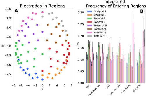
Figure 1: (A) Posizioni degli elettrodi per ciascuno dei 92 elettrodi sul copricapo di Electrical Geodesics Inc.. Gli elettrodi sono stati proiettati su un piano orizzontale con il naso nella direzione
positiva. Gli elettrodi sono stati codificati a colori per visualizzare le parti costituenti degli 8 gruppi per l'analisi della frequenza, vale a dire, occipitale sinistra (blu)/destra (arancione), parietale sinistra (verde)/destra (rosso), posteriore sinistra (viola)/ destra (marrone) e anteriore sinistra (rosa)/destra (grigio).
(B) Gli istogrammi che rappresentano la frequenza di ingresso in ciascuna regione fG vengono visualizzati per le sei condizioni testate. Un cambiamento significativo all'interno dello stimolo è presente tra ciascuna delle regioni anteriore sinistra e destra quando si confronta il riposo pre-stimolo e la rispettiva condizione stimolata (P < 0,001, modificata da Tukey). Le barre di errore mostrano l'intervallo di confidenza ad 1deviazione standard.
Spazio delle fasi
Abbiamo anche esplorato lo spazio delle fasi di valore medio di questo sistema. Lo spazio delle fasi per ciascun soggetto è stato tracciato come posizione media e momento lungo la direzione ,  oppure come posizione media e momento lungo la direzione ,
 .
.
La figura 2 mostra i centroidi dei grafici a dispersione dello spazio delle fasi per ciascun soggetto con un'ellisse che rappresenta l'intervallo di confidenza della deviazione standard. Si noti che i valori vengono riportati solo per gli stimoli intatti poiché un'analisi della varianza mostra che i film criptati e intatti sono indistinguibili nello spazio delle fasi ( , Tukey regolato). Le figure 2A e B mostrano la proiezione del baricentro dello spazio delle fasi sul piano attraversato da e
  per "Bang! Sei morto” e “Preso” rispettivamente, e Fig. 2C ed il piano D
  . La posizione media lungo l'asse
  per lo stimolo intatto ("BYD" e "Preso") e le loro forme criptate sono significativamente diverse dalle controparti di riposo pre-stimolo con (aggiustato da Tukey) mentre i centroidi di attività positivi e a riposo sono indistinguibili nel piano (
 , Tukey aggiustato).
Le medie del gruppo sono riportate nella Tabella Tabella 11 insieme alle loro deviazioni standard. Questi valori sono il valore medio dei centroidi (media dei punti centrali entro gli stimoli in Fig. 2) per la rispettiva posizione/momento all'interno di ciascun livello di stimolo. Come si vede anche in Fig. 2C e D, c'è una sorprendente differenza di un ordine di grandezza per  tra le condizioni di riposo e di attività, ma nessuna differenza marcata in ,
  o
o  .
.
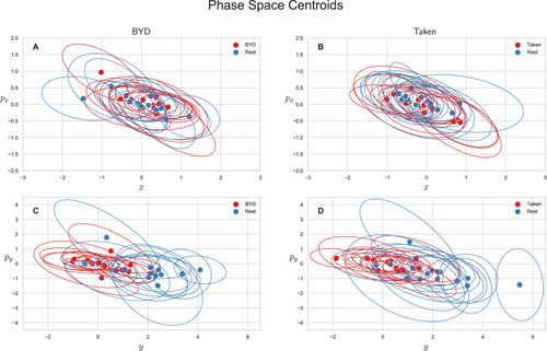
Figure 2: Centroidi medi dello spazio delle fasi per ciascun soggetto. Le ellissi rappresentano l'intervallo di confidenza della deviazione standard. I centroidi per gli stimoli codificati sono stati omessi in quanto non sono distinguibili dagli stimoli intatti (P > 0,85) (A) Centroidi per “Bang! Sei morto” lungo la direzione . (B) Centroidi per "Preso" lungo la direzione . (C) Centroidi per “Bang! Sei morto” lungo la direzione . (D) Centroidi per "Preso" lungo la direzione . Le differenze sono evidenti solo nella direzione (P < 0,001, modificato da Tukey) indicative del livello più elevato di attivazione anteriore come indicato in Fig. 1.. Tabella 1
Medie di gruppo dei centroidi.
| Stimulo
|

|
|
|
|
| Taken
|

|

|

|

|
| Taken Scrambled (destrutturato)
|

|

|

|

|
| Bang! You’re Dead
|

|

|

|

|
| Bang! You’re Dead (destrutturato)
|

|

|

|

|
| Rest (Pre-Taken)
|

|

|

|

|
| Rest (Pre-BYD)
|

|

|

|

|
Differenze significative si notano solo per la fase di riposto acquisito prima di Taken e Bang! Sei morto quando confrontati la posizione media con una delle loro controparti di attività (stimolo destrutturato e intatto).
Medie di gruppo dei centroidi.
Questa analisi ha rivelato due risultati notevoli. In primo luogo, c'era una mancanza di differenze significative nella quantità di moto del cervello lungo la direzione e . In secondo luogo, le medie dei momenti non erano significativamente diverse da 0 a livello di gruppo. I momenti positivi o negativi deriva dalla derivata temporale della probabilità e della posizione dell'elettrodo. Poiché la media dei momenti è 0, c'è un numero uguale di elettrodi anteriori e posteriori con probabilità sia in aumento che in diminuzione.
Inoltre, abbiamo esaminato i cambiamenti nei valori di probabilità sia nello stato di riposo che in quello attivo. Le animazioni delle distribuzioni di probabilità sono presenti nel materiale supplementare 1. In queste animazioni, le differenze di riposo e compito sono evidenti attraverso l'evoluzione della probabilità nel tempo.
Principio di indeterminazione
Nonostante la conferma dei precedenti risultati neuroscientifici e l'apparente successo del nostro modello quasi-quantistico, la nostra domanda di ricerca posta sopra rimane solo una risposta a metà. Utilizzando questo modello, abbiamo notato differenze nelle distribuzioni di probabilità e nei centroidi dello spazio delle fasi a riposo rispetto al compito. Tuttavia, abbiamo ancora cercato un parametro dal modello che sarebbe rimasto lo stesso in riposo e attività. A tal fine, abbiamo definito un analogo principio di indeterminazione di Heisenberg della forma,
|
|

|

|
La tabella 2 mostra i valori di questa costante () acquisiti in tutte le condizioni, nonché il valore massimo, il valore medio e la deviazione standard. Abbiamo scoperto che questo modello quasi-quantistico porta a un valore minimo costante su  e
e di
di  con
con  .
.
Si noti che l'unità di  è il risultato del campionamento dell'EEG a 250 Hz e della massa considerata come unità. Inoltre, il valore medio e la deviazione standard di queste quantità rimangono coerenti tra le condizioni con un valore medio di
  () e una deviazione standard di
  ).
).
In particolare, il valore massimo varia tra le condizioni, con il valore più grande che si verifica mentre i soggetti guardavano la clip intatta di Bang! Sei morto. Nonostante la posizione media del segnale lungo la direzione sia diversa a riposo rispetto a un compito (), la metodologia matematica quasi quantistica porta a un valore di incertezza costante. Abbastanza sorprendentemente, i valori nella tabella mostrano che l'incertezza media e l'incertezza minima sono le stesse in condizioni diverse, nonostante i massimi varino di oltre due ordini di grandezza. Pertanto, dando ulteriore credito all'idea che questa relazione di incertezza coglie le somiglianze del cervello in condizioni molto diverse. La Figura 3 mostra la distribuzione di probabilità al momento corrispondente al minimo di incertezza sia per che per .
Tabella 2
Considerando il valore minimo che questi prodotti raggiungono per ogni soggetto, vediamo un valore costante sia in x che in y di , un valore medio di e una deviazione standard costante di . L'unità di deriva dal campionamento di 250 Hz. I valori massimi differiscono a seconda della stimolazione. I valori sono riportati come media tra soggetti più o meno 1 deviazione standard.
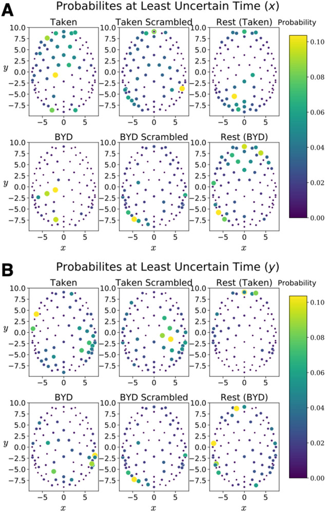
Figura 3: Mappe di probabilità corrispondenti al punto temporale meno incerto per ciascuna delle sei condizioni sperimentali. (A) Le probabilità che portano all'incertezza minima definita dal minimo di . (B) Le probabilità che portano all'incertezza minima definita dal minimo di . (B) Le probabilità che portano all'incertezza minima definita dal minimo di .Viene visualizzato un soggetto per tutti gli stimoli Taken ed un altro per tutti gli stimoli Bang! Sei morto. Discussion
Nel presente studio, abbiamo studiato l'estensione spaziale e le proprietà di transizione associate dell'attività neurale nel cervello durante condizioni attive e di riposo e se esistono proprietà di rete sottostanti simili. Abbiamo scoperto che l'applicazione della trasformata di Hilbert ai dati EEG e la sua normalizzazione (Eq. 2) impone una struttura probabilistica al segnale EEG attraverso il cervello (Eq. 3), che abbiamo usato per identificare la probabilità dei modelli spaziali di attività insieme alle transizioni in attività su tutto il cuoio capelluto. Abbiamo riscontrato una maggiore attività anteriore durante il riposo rispetto alla visione del film, sia nell'ampiezza che nello spazio delle fasi. Questo risultato è in linea con i risultati precedenti che mostrano una maggiore attivazione nella regione anteriore durante il riposo.[14][22][54][57][58] Inoltre, normalizzando i segnali EEG con le trasformate di Hilbert ed estraendo valori medi simili a quelli della formulazione della funzione d'onda della meccanica quantistica, siamo stati in grado di calcolare l'incertezza nella "posizione" e nei "momenti" durante il riposo e la visione di film, settata in una nuova costante denominata 
È allettante associare la costante relativa alla "posizione" e al "momento" dell'attività neurale a un principio fondamentale, come il principio di indeterminazione di Heisenberg. Tuttavia, non è ancora chiaro cosa significhi questa incertezza. Potrebbe implicare limiti al grado in cui il cervello è accessibile; l'aumento delle informazioni sulla posizione precisa dello stato cerebrale (come descritto dalle nostre "funzioni d'onda" quasi quantistiche) aumenterà l'incertezza su dove sarà in un momento successivo. Questi risultati offrono una prospettiva interessante sul legame tra funzione neurale e processi cognitivi. Ad esempio, quando la "funzione d'onda" si localizza nello spazio lungo un treno di pensieri, ci distraiamo per aumentare l'incertezza, il che potrebbe spiegare perché le menti vagano e i pensieri sono fugaci?
Il valore  che abbiamo trovato è costante in diverse condizioni di stimolo e indipendente dal numero di elettrodi utilizzati per acquisire i dati? Per testare questo, abbiamo campionato gli elettrodi EEG da 92 a 20 ed eseguito la stessa analisi del testo principale. In linea con 92 canali, abbiamo riscontrato la tendenza anteriore a riposo, ma abbiamo riscontrato che riducendo gli elettrodi a 20 risultava una costante differente
  (Vedi materiale supplementare). Ciò dimostra che il modello è in grado di catturare le differenze di riposo/attività ma potrebbe essere necessario introdurre una condizione di normalizzazione dipendente dal montaggio.
È importante notare che i valori di incertezza di questa forma sono inerenti a qualsiasi variabile coniugata di Fourier, poiché un valore si diffonde in una variabile e si localizza nell'altra. Ciò suggerisce che dopo aver definito il quadrato dell'andamento temporale dell'elettrodo EEG nella trasformata di Hilbert come probabilità ed aver imposto le proprietà di uno spazio di Hilbert sui segnali dell'elettrodo, è possibile estrarre valori di incertezza. Nella meccanica quantistica, questa incertezza stabilisce il limite per le scale che non possono essere osservate. Questo approccio è stato ispirato dalla necessità nelle neuroscienze di nuovi modelli per aiutare a interpretare i dati di neuroimaging. Sebbene questo sia un interessante passo avanti metodologico, dobbiamo comunque determinare se l'incertezza osservata nei dati EEG è supportata da un nuovo principio fondamentale come nella meccanica quantistica o se è solo il risultato di aver costruito due nuove variabili coniugate di Fourier dal Segnale EEG.
È necessario fare ulteriore lavoro per esplorare questa costante rispetto alla ricca tassonomia di compiti e stimoli e ai vari stati di coscienza che sono abitualmente utilizzati nelle neuroscienze cognitive. Questa metodologia potrebbe essere estesa alla fMRI, dove i percorsi temporali BOLD potrebbero essere trasformate di Hilbert creando un analogo tridimensionale del modello EEG presentato in questo articolo.
In definitiva, questo documento ha presentato una nuova metodologia per l'analisi dei dati EEG. Normalizzare i dati e trattarli come un'ampiezza di probabilità ha portato a parametri che cambiavano con la presenza o la mancanza di stimolo, stabilendo contemporaneamente un valore costante indipendente dallo stimolo. Abbiamo applicato con successo un quadro matematico basato sui formalismi della meccanica quantistica al paradigma del riposo e del compito nell'EEG (senza pretendere che il cervello sia un oggetto quantistico). Poiché la neuroscienza continua ad evolversi, anche gli strumenti analitici a sua disposizione devono progredire di conseguenza. Ci auguriamo che questo strumento analitico, insieme ai progressi nella modellazione e nell'apprendimento automatico, aiutino a comprendere la natura della coscienza.
È importante notare che i valori di incertezza di questa forma sono inerenti a qualsiasi variabile coniugata di Fourier, poiché un valore si diffonde in una variabile, si localizza nell'altra. Ciò suggerisce che dopo aver definito il quadrato dell'andamento temporale dell'elettrodo EEG trasformato di Hilbert come probabilità e aver imposto le proprietà di uno spazio di Hilbert sui segnali dell'elettrodo, è possibile estrarre valori di incertezza. Nella meccanica quantistica, questa incertezza stabilisce il limite per le scale che non possono essere osservate. Questo approccio è stato ispirato dalla necessità nelle neuroscienze di nuovi modelli per aiutare a interpretare i dati di neuroimaging. Sebbene questo sia un interessante passo avanti metodologico, dobbiamo comunque determinare se l'incertezza osservata nei dati EEG è supportata da un nuovo principio fondamentale come nella meccanica quantistica, o se è solo il risultato di aver costruito due nuove variabili coniugate di Fourier dal Segnale EEG.
È necessario fare ulteriore lavoro per esplorare questa costante rispetto alla ricca tassonomia di compiti e stimoli e ai vari stati di coscienza che sono abitualmente utilizzati nelle neuroscienze cognitive. Questa metodologia potrebbe essere estesa alla fMRI, dove i corsi temporali BOLD potrebbero essere trasformati da Hilbert creando un analogo tridimensionale del modello EEG presentato in questo articolo.
In definitiva, questo documento ha presentato una nuova metodologia per l'analisi dei dati EEG. Normalizzare i dati e trattarli come un'ampiezza di probabilità ha portato a parametri che cambiavano con la presenza o la mancanza di stimolo, stabilendo contemporaneamente un valore costante indipendente dallo stimolo. Abbiamo applicato con successo un quadro matematico basato sui formalismi della meccanica quantistica al paradigma del riposo e del compito nell'EEG (senza pretendere che il cervello sia un oggetto quantistico). Poiché la neuroscienza continua ad evolversi, anche gli strumenti analitici a sua disposizione devono progredire di conseguenza. Ci auguriamo che questo strumento analitico, insieme ai progressi nella modellazione e nell'apprendimento automatico, aiutino a comprendere la natura della coscienza.
Metodi
Acquisizione dati
Ventotto soggetti sani sono stati reclutati dal Brain and Mind Institute dell'Università dell'Ontario occidentale, in Canada, per partecipare a questo studio. Il consenso scritto informato è stato acquisito prima del test da tutti i partecipanti. L'approvazione etica per questo studio è stata concessa dall'Health Sciences Research Ethics Board e dal Non-Medical Research Ethics Board dell'Università dell'Ontario occidentale e tutta la ricerca è stata eseguita in conformità con le linee guida/normative pertinenti e in conformità con la Dichiarazione di Helsinki.
Due filmati pieni di suspense sono stati usati come stimoli naturalistici in questo studio. Un videoclip dal film muto “Bang! You're Dead" ( Bang! Tu sei morto) e un estratto audio dal film "Taken" sono stati mostrati rispettivamente a 13 e 15 soggetti nelle loro forme originali intatte e distorte. Prima delle due acquisizioni, è stata acquisita una sezione di riposo in cui ai soggetti è stato chiesto di rilassarsi, senza alcuna stimolazione evidente. La presentazione dello stimolo è stata controllata con il plug-in Psychtoolbox per MATLAB[38][38][59][60] su un Apple MacBook Pro da 15″.[61] L'audio è stato presentato in modo binaurale a un volume di ascolto confortevole tramite le cuffie Etymotics ER-1.
I dati EEG sono stati raccolti utilizzando un cuffia a 129 canali (Electrical Geodesics Inc. [EGI], Oregon, USA). Le impedenze degli elettrodi sono state mantenute al di sotto di 50 kΩ con segnali campionati a 250 Hz e riferiti al vertice centrale (Cz). Utilizzando il toolbox EEGLAB MATLAB, i canali rumorosi sono stati identificati e rimossi, quindi interpolati nuovamente nei dati. Un test Kolmogorov-Smirnov (KS) sui dati è stato utilizzato per identificare le regioni che non erano gaussiane. L'analisi delle componenti indipendenti (ICA) è stata quindi utilizzata per identificare visivamente i modelli di attività neurale caratteristici dei movimenti oculari e muscolari che sono stati successivamente rimossi dai dati. La pre-elaborazione dell'EEG è stata eseguita individualmente per ogni soggetto e condizione.
Dei due filmati testati, il primo era un segmento di 8 minuti del film muto televisivo di Alfred Hitchcock “Bang! Sei morto". Questa scena ritrae un bambino di 5 anni che prende in mano la rivoltella di suo zio. Il ragazzo carica un proiettile nella pistola e ci gioca come se fosse un giocattolo. Il ragazzo (e lo spettatore) raramente sa se la pistola ha un proiettile nella sua camera e la suspense aumenta quando il ragazzo gira la camera, la punta verso gli altri e preme il grilletto. In alternativa alla stimolazione visiva, è stato utilizzato anche un estratto audio di 5 minuti dal film "Taken". Questa clip ritrae una conversazione telefonica in cui un padre sente per caso il rapimento delle sue figlie.
Inoltre, sono stati utilizzati due stimoli di controllo "criptati", uno per ogni film. Questo separa le risposte neurali suscitate dalle proprietà sensoriali della visione o dell'ascolto dei film da quelle coinvolte nel seguire la trama. La versione distorta di “Bang! You're Dead" è stato generato isolando i segmenti di 1s mescolando in modo pseudocasuale i segmenti, eliminando così la coerenza temporale della narrazione.[38][62] La versione criptata di "Taken" è stata creata ruotando spettralmente l'audio, rendendo così il discorso indecifrabile.[62][63] I filmati distorti sono stati presentati prima delle versioni intatte per evitare potenziali effetti di trascinamento della narrazione. Prima che i soggetti guardassero/ascoltassero lo stimolo codificato, veniva acquisito un breve segmento di EEG a riposo.
Modello
Ciascuno degli elettrodi è descritto da una coppia ordinata  nello spazio tridimensionale. Per completare questa analisi, gli elettrodi sono stati prima proiettati sul piano
  , rimuovendo la profondità della testa. La figura 1A mostra le posizioni di ciascun elettrodo in questo spazio
  . A seguito di questa proiezione, gli andamenti temporali per ciascuno dei 92 elettrodi sono stati trasformate di Hilbert e quindi normalizzati secondo la procedura elencata utilizzando l'Eq. (2). Una probabilità è stata definita in questo spazio di posizione degli elettrodi come il quadrato dell'andamento temporale della trasformata di Hilbert (Eq. 3), analogo alle funzioni d'onda della meccanica quantistica. Otto regioni (L/R anteriore, L/R posteriore, L/R parietale, L/R occipitale) sono state quindi definite raggruppando i 92 elettrodi e le frequenze di ingresso in ciascuna regione fG sono state ottenute sommando le probabilità degli elettrodi all'interno del gruppo, poi integrandosi nel tempo.
|
|

|

|
dove ciascuno degli otto gruppi indicati dal pedice ha un numero diverso di elettrodi costituenti N. Nell'occipite sinistro e destro ci sono 10 elettrodi ciascuno, nel parietale sinistro e destro ci sono 17 elettrodi ciascuno, nel posteriore sinistro e destro ci sono rispettivamente 10 e 11 elettrodi, e nella parte anteriore sinistra e destra ci sono rispettivamente 8 e 9 elettrodi.
Dopo aver ottenuto le frequenze a livello di gruppo, i valori medi per posizione e quantità di moto sono stati calcolati utilizzando le equazioni. (4) e (5) (con espressioni identiche per ). Infine, per accertare il nostro analogo principio di indeterminazione, abbiamo cercato espressioni della forma
|
|

|

|
L'espressione for può essere prontamente applicata alle probabilità e posizioni come sopra definite, risultando nel primo termine dato da
|
|

|

|
E il secondo termine dato dal quadrato dell'Eq. (4). Il secondo termine di  è dato dal quadrato dell'Eq. (5), ma il primo termine è più sfumato. Ciò è dovuto al numero complesso restituito quando si agisce due volte sull'operatore derivato sulla probabilità. Per ovviare a questo, le trasformate di Fourier sono state utilizzate per cambiare l'Eq. (5) nella base della quantità di moto che ha quindi consentito il calcolo efficiente di
  .
.
Indicando 0 come la probabilità dello spazio di moto ottenuta attraverso una trasformata di Fourier bidimensionale e non uniforme della pseudo-funzione d'onda dello spazio delle posizioni, l'Eq. (5) può essere riscritto come,
Indicando  come la probabilità dello spazio di moto ottenuta attraverso una trasformata di Fourier bidimensionale e non uniforme della pseudo-funzione d'onda dello spazio delle posizioni, l'Eq. (5) può essere riscritto come,
|
|

|

|
Portando al primo termine nell'espressione da scrivere come,
|
|
![{\displaystyle \langle p_{x}^{2}(t)\rangle =m^{2}\sum _{j=1}^{92}{\tfrac {x_{j}^{2}}{{\tilde {p}}_{j}(t)}}[{d \over dt}P_{j}(t)]^{2}}](https://wikimedia.org/api/rest_v1/media/math/render/svg/3dda471e5a09b53812126091bf6b9a73fc19a4f4)
|

|
Il wrapper Python FINUFFT è stato utilizzato per prendere la trasformata di Fourier utilizzando un tipo 3, 2d FFT non uniforme,[64][65] ed è stato trovato il valore minimo nel tempo della relazione di incertezza. I punti nello spazio della quantità di moto sono stati campionati su ![{\displaystyle p_{x}\in [-4,4]}](https://wikimedia.org/api/rest_v1/media/math/render/svg/515f4df54a0052df61a308afa0bb41739bf89ef0) e
e ![{\displaystyle p_{y}\in [-4,5]}](https://wikimedia.org/api/rest_v1/media/math/render/svg/950ccba52979e32d86080daf5a94cb3b5524feb6) insieme ai due punti aggiuntivi (
insieme ai due punti aggiuntivi (![{\displaystyle [-5,-4]}](https://wikimedia.org/api/rest_v1/media/math/render/svg/c1acb0cb7df6bce649ff45049f7f85ca28c1c5b7) ) e (
) e (![{\displaystyle [-4,-5]}](https://wikimedia.org/api/rest_v1/media/math/render/svg/c01ceeb13f42e4e0cc0444eefecc2e668333a503) )
)
La figura 4 mostra rispettivamente le probabilità di posizione e quantità di moto nella loro base. Un'animazione che mostra come questi si evolvono nel tempo per le diverse condizioni è presentata nel materiale supplementare 2.
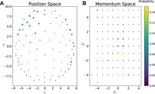
Figure 4: (A) Distribuzione di probabilità per un singolo soggetto in base alla posizione. (B) Distribuzione di probabilità basata sulla quantità di moto per un singolo soggetto. I valori di quantità di moto utilizzati per la trasformata di Fourier sono indicati dalle posizioni dei punti. I punti sono codificati per colore/dimensione per rappresentare il valore di probabilità in quella posizione. Per calcolare i valori riportati nella tabella 2, è stato trovato il valore corrispondente per ciascun soggetto e questi sono stati utilizzati per calcolare la media di gruppo qui riportata.
Informazioni supplementari
Supplementary Figures.(28M, docx)
Supplementary Information.(375K, docx)
Acknowledgements
We would like to thank Silvano Petrarca for his continued assistance in devising the model. This study was funded by the NSERC Discovery Grant (05578–2014RGPIN), CERC (215063), CIHR Foundation Fund (167264). AMO is a Fellow of the CIFAR Brain, Mind, and Consciousness Program.
Author contributions
N.J.M.P., C.M. and G.L. performed the analysis. A.S., B.S. and N.J.M.P. developed the model. A.S. and B.S. supervised the analysis. N.J.M.P., A.S., G.L. and B.S. wrote the manuscript. A.M.O. revised the manuscript.
Competing interests
The authors declare no competing interests.
Publisher's note
Springer Nature remains neutral with regard to jurisdictional claims in published maps and institutional affiliations.
These authors contributed equally: Bobby Stojanoski and Andrea Soddu.
Supplementary Information
The online version contains supplementary material available at 10.1038/s41598-021-97960-7.
Article information
Sci Rep. 2021; 11: 19771.
Published online 2021 Oct 5. doi: 10.1038/s41598-021-97960-7
PMCID: PMC8492705
PMID: 34611185
Nicholas J. M. Popiel,1,2 Colin Metrow,1 Geoffrey Laforge,3 Adrian M. Owen,3,4,5 Bobby Stojanoski,#4,6 and Andrea Soddu#1,3
1The Department of Physics and Astronomy, The University of Western Ontario, London, ON N6A 5B7 Canada
2Cavendish Laboratory, University of Cambridge, Cambridge, CB3 0HE UK
3The Brain and Mind Institute, The University of Western Ontario, London, ON N6A 5B7 Canada
4The Department of Psychology, The University of Western Ontario, London, ON N6A 5B7 Canada
5The Department of Physiology and Pharmacology, The University of Western Ontario, London, ON N6A 5B7 Canada
6Faculty of Social Science and Humanities, University of Ontario Institute of Technology, 2000 Simcoe Street North, Oshawa, ON L1H 7K4 Canada
Andrea Soddu, Email: asoddu@uwo.ca
Corresponding author.
- Contributed equally.
Received 2021 Apr 28; Accepted 2021 Aug 30.
Copyright © The Author(s) 2021
Open Access
This article is licensed under a Creative Commons Attribution 4.0 International License, which permits use, sharing, adaptation, distribution and reproduction in any medium or format, as long as you give appropriate credit to the original author(s) and the source, provide a link to the Creative Commons licence, and indicate if changes were made. The images or other third party material in this article are included in the article's Creative Commons licence, unless indicated otherwise in a credit line to the material. If material is not included in the article's Creative Commons licence and your intended use is not permitted by statutory regulation or exceeds the permitted use, you will need to obtain permission directly from the copyright holder. To view a copy of this licence, visit http://creativecommons.org/licenses/by/4.0/.
Articles from Scientific Reports are provided here courtesy of == Nature Publishing Group ==
Bibliography & references
- ↑ Biswal B, Zerrin Yetkin F, Haughton VM, Hyde JS, «Functional connectivity in the motor cortex of resting human brain using echo-planar MRI», in Magn Reson Med, 1995».
PMID:8524021
DOI:10.1002/mrm.1910340409
- ↑ Hutchison RM, Womelsdorfb T, Allenc EA, Bandettini PA, Calhound VD, Corbetta M, Della Penna S, «Dynamic functional connectivity: Promise, issues, and interpretations», in Neuroimage, 2013».
PMID:23707587 - PMCID:PMC3807588
DOI:10.1016/j.neuroimage.2013.05.079
- ↑ Eickhoff SB, Yeo BTT, Genon S, «Imaging-based parcellations of the human brain», in Nat Rev Neurosci, 2018».
PMID:30305712
DOI:10.1038/s41583-018-0071-7
- ↑ Dajani DR, Burrows CA, Odriozola P, Baez A, Nebel MB, Mostofsky SH, Uddin LQ, «Investigating functional brain network integrity using a traditional and novel categorical scheme for neurodevelopmental disorders», in NeuroImage Clin, 2019».
PMID:30708240 - PMCID:PMC6356009
DOI:10.1016/j.nicl.2019.101678
- ↑ Uddin LQ, Karlsgodt KH, «Future directions for examination of brain networks in neurodevelopmental disorders», in J Clin Child Adolesc Psychol, Society of Clinical Child & Adolescent Psychology, 2018».
PMID:29634380 - PMCID:PMC6842321
DOI:10.1080/15374416.2018.1443461
- ↑ Sripada C, Rutherford S, Angstadt M, Thompson WK, Luciana M, Weigard A, Hyde LH, «Prediction of neurocognition in youth from resting state fMRI», in Mol Psychiatry, 2020».
PMID:31427753 - PMCID:PMC7055722
DOI:10.1038/s41380-019-0481-6
- ↑ Biswal BB, Eldreth DA, Motes MA, Rypma B, «Task-dependent individual differences in prefrontal connectivity», in Cereb Cortex, Oxford University Press, 2010, Oxford, UK».
PMID:20064942 - PMCID:PMC2923215
DOI:10.1093/cercor/bhp284
|
|
This is an Open Access resource!
|
- ↑ Fox MD, Raichle ME, «Spontaneous fluctuations in brain activity observed with functional magnetic resonance imaging», in Nat Rev Neurosci, 2007».
PMID:17704812
DOI:10.1038/nrn2201
- ↑ Kraus Brian T, Perez Diana, Ladwig Zach, Seitzman Benjamin A, Dworetsky Ally, Petersen Steven E, Gratton Caterina, «Network variants are similar between task and rest states», in Neuroimage, 2021».
PMID:33454409 - PMCID:PMC8080895
DOI:10.1016/j.neuroimage.2021.117743
|
|
This is an Open Access resource!
|
- ↑ Kristo Gert, Rutten Geert-Jan, Raemaekers Mathijs, de Gelder Bea, Rombouts Serge ARB, Ramsey Nick F, «Task and task-free FMRI reproducibility comparison for motor network identification», in Hum Brain Mapp, 2014».
PMID:22987751 - PMCID:PMC6869575
DOI:10.1002/hbm.22180
- ↑ Sui J, Adali T, Pearlson GD, Calhoun VD, «An ICA-based method for the identification of optimal FMRI features and components using combined group-discriminative techniques», in Neuroimage, 2009».
PMID:19457398 - PMCID:PMC4356027
DOI:10.1016/j.neuroimage.2009.01.026
- ↑ Calhoun VD, Kiehl KA, Pearlson GD, «Modulation of temporally coherent brain networks estimated using ICA at rest and during cognitive tasks», in Hum Brain Mapp, 2008».
PMID:18438867 - PMCID:PMC2649823
DOI:10.1002/hbm.20581
- ↑ Xie Hua, Calhoun Vince D, Gonzalez-Castillo Javier, Damaraju Eswar, Miller Robyn, Bandettini Peter A, Mitra Sunanda, «Whole-brain connectivity dynamics reflect both task-specific and individual-specific modulation: A multitask study», in Neuroimage, 2018».
PMID:28549798 - PMCID:PMC5700856
DOI:10.1016/j.neuroimage.2017.05.050
- ↑ 14.0 14.1 Naci L, Cusack R, Anello M, Owen AM, «A common neural code for similar conscious experiences in different individuals», in Proc Natl Acad Sci, 2014».
PMID:25225384 - PMCID:PMC4191782
DOI:10.1073/pnas.1407007111
- ↑ Kannurpatti SS, Rypma B, Biswal BB, «Prediction of task-related BOLD fMRI with amplitude signatures of resting-state fMRI», in Front Syst Neurosci, 2012».
PMID:22408609 - PMCID:PMC3294272
DOI:10.3389/fnsys.2012.00007
- ↑ Elliott Maxwell L, Knodt Annchen R, Cooke Megan, Kim M Justin, Melzer Tracy R, Keenan Ross, Ireland David, «General functional connectivity: Shared features of resting-state and task fMRI drive reliable and heritable individual differences in functional brain networks», in Neuroimage, 2019».
PMID:30708106 - PMCID:PMC6462481
DOI:10.1016/j.neuroimage.2019.01.068
- ↑ Cole MW, Ito T, Cocuzza C, Sanchez-Romero R, «The functional relevance of task-state functional connectivity», in Neurosci, 2021».
PMID:33542083 - PMCID:PMC8018740
DOI:10.1523/JNEUROSCI.1713-20.2021
- ↑ Zhang Shu, Li Xiang, Lv Jinglei, Jiang Xi, Guo Lei, Liu Tianming, «Characterizing and differentiating task-based and resting state fMRI signals via two-stage sparse representations», in Brain Imaging Behav, 2016».
PMID:25732072 - PMCID:PMC4559495
DOI:10.1007/s11682-015-9359-7
- ↑ Monier C, Chavane F, Baudot P, Graham LJ, Frégnac Y, «Orientation and direction selectivity of synaptic inputs in visual cortical neurons: A diversity of combinations produces spike tuning», in Neuron, 2003».
PMID:12597863
DOI:10.1016/S0896-6273(03)00064-3
- ↑ Churchland MM, et al. Stimulus onset quenches neural variability: A widespread cortical phenomenon. Nat. Neurosci. 2010;13:369–378. doi: 10.1038/nn.2501. [PMC free article][PubMed] [CrossRef] [Google Scholar]
- ↑ He BJ. Spontaneous and task-evoked brain activity negatively interact. J. Neurosci. 2013;33:4672–4682. doi: 10.1523/JNEUROSCI.2922-12.2013. [PMC free article][PubMed] [CrossRef] [Google Scholar]
- ↑ 22.0 22.1 22.2 22.3 Bonnard M, et al. Resting state brain dynamics and its transients: A combined TMS-EEG study. Sci. Rep. 2016;6:1–9. doi: 10.1038/srep31220. [PMC free article] [PubMed] [CrossRef] [Google Scholar]
- ↑ 23.0 23.1 23.2 Axelrod V, Zhu X, Qiu J. Transcranial stimulation of the frontal lobes increases propensity of mind-wandering without changing meta-awareness. Sci. Rep. 2018;8:1–14. doi: 10.1038/s41598-018-34098-z. [PMC free article] [PubMed] [CrossRef] [Google Scholar]
- ↑ 24.0 24.1 24.2 24.3 Axelrod V, Rees G, Lavidor M, Bar M. Increasing propensity to mind-wander with transcranial direct current stimulation. Proc. Natl. Acad. Sci. U. S. A. 2015;112:3314–3319. doi: 10.1073/pnas.1421435112. [PMC free article] [PubMed] [CrossRef] [Google Scholar]
- ↑ 25.0 25.1 25.2 Townsend JS. A Modern Approach to Quantum Mechanics.University Science Books; 2012. [Google Scholar]
- ↑ Heisenberg W. Über den anschaulichen Inhalt der quantentheoretischen Kinematik und Mechanik. Z. Phys. 1927;43:172–198. doi: 10.1007/BF01397280. [CrossRef] [Google Scholar]
- ↑ Penrose R. The Emperor’s New Mind. Viking Penguin; 1990. [Google Scholar]
- ↑ Penrose R. Shadows of the Mind: A Search for the Missing Science of Consciousness. Oxford University Press; 1994. [Google Scholar]
- ↑ Atmanspacher H. Quantum Approaches to Consciousness.Stanford Encyclopedia of Philosophy; 2004. [Google Scholar]
- ↑ Hameroff S. How quantum brain biology can rescue conscious free will. Front. Integr. Neurosci. 2012;6:93. doi: 10.3389/fnint.2012.00093. [PMC free article] [PubMed] [CrossRef] [Google Scholar]
- ↑ Biswal BB, Eldreth DA, Motes MA, Rypma B. Task-dependent individual differences in prefrontal connectivity. Cereb. Cortex. 2010;20:2188–2197. doi: 10.1093/cercor/bhp284. [PMC free article][PubMed] [CrossRef] [Google Scholar]
- ↑ Fox MD, Raichle ME. Spontaneous fluctuations in brain activity observed with functional magnetic resonance imaging. Nat. Rev. Neurosci. 2007;8:700–711. doi: 10.1038/nrn2201. [PubMed] [CrossRef] [Google Scholar]
- ↑ Kraus BT, et al. Network variants are similar between task and rest states. Neuroimage. 2021;229:117743. doi: 10.1016/j.neuroimage.2021.117743. [PMC free article][PubMed] [CrossRef] [Google Scholar]
- ↑ Kristo G, et al. Task and task-free FMRI reproducibility comparison for motor network identification. Hum. Brain Mapp. 2014;35:340–352. doi: 10.1002/hbm.22180. [PMC free article][PubMed] [CrossRef] [Google Scholar]
- ↑ Sui J, Adali T, Pearlson GD, Calhoun VD. An ICA-based method for the identification of optimal FMRI features and components using combined group-discriminative techniques. Neuroimage. 2009;46:73–86. doi: 10.1016/j.neuroimage.2009.01.026.[PMC free article] [PubMed] [CrossRef] [Google Scholar]
- ↑ Calhoun VD, Kiehl KA, Pearlson GD. Modulation of temporally coherent brain networks estimated using ICA at rest and during cognitive tasks. Hum. Brain Mapp. 2008;29:828–838. doi: 10.1002/hbm.20581. [PMC free article] [PubMed] [CrossRef] [Google Scholar]
- ↑ Xie H, et al. Whole-brain connectivity dynamics reflect both task-specific and individual-specific modulation: A multitask study. Neuroimage. 2018;180:495–504. doi: 10.1016/j.neuroimage.2017.05.050. [PMC free article] [PubMed] [CrossRef] [Google Scholar]
- ↑ 38.0 38.1 38.2 38.3 Naci L, Cusack R, Anello M, Owen AM. A common neural code for similar conscious experiences in different individuals. Proc. Natl. Acad. Sci. U. S. A. 2014;111:14277–14282. doi: 10.1073/pnas.1407007111. [PMC free article] [PubMed] [CrossRef] [Google Scholar] Cite error: Invalid
<ref> tag; name ":0" defined multiple times with different content
- ↑ Kannurpatti SS, Rypma B, Biswal BB. Prediction of task-related BOLD fMRI with amplitude signatures of resting-state fMRI. Front. Syst. Neurosci. 2012;6:7. doi: 10.3389/fnsys.2012.00007.[PMC free article] [PubMed] [CrossRef] [Google Scholar]
- ↑ Elliott ML, et al. General functional connectivity: Shared features of resting-state and task fMRI drive reliable and heritable individual differences in functional brain networks. Neuroimage. 2019;189:516–532. doi: 10.1016/j.neuroimage.2019.01.068. [PMC free article][PubMed] [CrossRef] [Google Scholar]
- ↑ Cole MW, Ito T, Cocuzza C, Sanchez-Romero R. The functional relevance of task-state functional connectivity. J. Neurosci. 2021 doi: 10.1523/JNEUROSCI.1713-20.2021. [PMC free article][PubMed] [CrossRef] [Google Scholar]
- ↑ Zhang S, et al. Characterizing and differentiating task-based and resting state fMRI signals via two-stage sparse representations. Brain Imaging Behav. 2016;10:21–32. doi: 10.1007/s11682-015-9359-7.[PMC free article] [PubMed] [CrossRef] [Google Scholar]
- ↑ Monier C, Chavane F, Baudot P, Graham LJ, Frégnac Y. Orientation and direction selectivity of synaptic inputs in visual cortical neurons: A diversity of combinations produces spike tuning. Neuron. 2003;37:663–680. doi: 10.1016/S0896-6273(03)00064-3.[PubMed] [CrossRef] [Google Scholar]
- ↑ Churchland MM, et al. Stimulus onset quenches neural variability: A widespread cortical phenomenon. Nat. Neurosci. 2010;13:369–378. doi: 10.1038/nn.2501. [PMC free article][PubMed] [CrossRef] [Google Scholar]
- ↑ He BJ. Spontaneous and task-evoked brain activity negatively interact. J. Neurosci. 2013;33:4672–4682. doi: 10.1523/JNEUROSCI.2922-12.2013. [PMC free article][PubMed] [CrossRef] [Google Scholar]
- ↑ Heisenberg W. Über den anschaulichen Inhalt der quantentheoretischen Kinematik und Mechanik. Z. Phys. 1927;43:172–198. doi: 10.1007/BF01397280. [CrossRef] [Google Scholar]
- ↑ Penrose R. The Emperor’s New Mind. Viking Penguin; 1990. [Google Scholar]
- ↑ Penrose R. Shadows of the Mind: A Search for the Missing Science of Consciousness. Oxford University Press; 1994. [Google Scholar]
- ↑ Atmanspacher H. Quantum Approaches to Consciousness.Stanford Encyclopedia of Philosophy; 2004. [Google Scholar]
- ↑ Hameroff S. How quantum brain biology can rescue conscious free will. Front. Integr. Neurosci. 2012;6:93. doi: 10.3389/fnint.2012.00093. [PMC free article] [PubMed] [CrossRef] [Google Scholar]
- ↑ Freeman WJ, Vitiello G. Nonlinear brain dynamics as macroscopic manifestation of underlying many-body field dynamics. Phys. Life Rev. 2006;3:93–118. doi: 10.1016/j.plrev.2006.02.001.[CrossRef] [Google Scholar]
- ↑ le Van Quyen M, et al. Comparison of Hilbert transform and wavelet methods for the analysis of neuronal synchrony. J. Neurosci. Methods. 2001;111:83–98. doi: 10.1016/S0165-0270(01)00372-7.[PubMed] [CrossRef] [Google Scholar]
- ↑ Freeman WJ. Deep analysis of perception through dynamic structures that emerge in cortical activity from self-regulated noise. Cogn. Neurodyn. 2009;3:105–116. doi: 10.1007/s11571-009-9075-3.[PMC free article] [PubMed] [CrossRef] [Google Scholar]
- ↑ 54.0 54.1 Wang RWY, Chang WL, Chuang SW, Liu IN. Posterior cingulate cortex can be a regulatory modulator of the default mode network in task-negative state. Sci. Rep. 2019;9:1–12. [PMC free article][PubMed] [Google Scholar]
- ↑ Uddin LQ, Kelly AMC, Biswal BB, Castellanos FX, Milham MP. Functional connectivity of default mode network components: Correlation, anticorrelation, and causality. Hum. Brain Mapp. 2009;30:625–637. doi: 10.1002/hbm.20531. [PMC free article][PubMed] [CrossRef] [Google Scholar]
- ↑ Stawarczyk D, Majerus S, Maquet P, D’Argembeau A. Neural correlates of ongoing conscious experience: Both task-unrelatedness and stimulus-independence are related to default network activity. PLoS One. 2011;6:e16997. doi: 10.1371/journal.pone.0016997.[PMC free article] [PubMed] [CrossRef] [Google Scholar]
- ↑ 57.0 57.1 Greicius, M. D., Krasnow, B., Reiss, A. L., Menon, V. & Raichle, M. E. Functional Connectivity in the Resting Brain: A Network Analysis of the Default Mode Hypothesis. www.pnas.org. [PMC free article] [PubMed]
- ↑ Christoff K, Gordon AM, Smallwood J, Smith R, Schooler JW. Experience sampling during fMRI reveals default network and executive system contributions to mind wandering. Proc. Natl. Acad. Sci. U. S. A. 2009;106:8719–8724. doi: 10.1073/pnas.0900234106.[PMC free article] [PubMed] [CrossRef] [Google Scholar]
- ↑ Kleiner M, et al. What’s new in psychtoolbox-3. Perception. 2007;36:1–16. [Google Scholar]
- ↑ Pelli DG. The VideoToolbox software for visual psychophysics: Transforming numbers into movies. Spat. Vis. 1997;10:437–442. doi: 10.1163/156856897X00366. [PubMed] [CrossRef] [Google Scholar]
- ↑ Makeig, S. & Onton, J. ERP features and EEG dynamics: An ICA perspective. In The Oxford Handbook of Event-Related Potential Components (Oxford University Press, 2012). 10.1093/oxfordhb/9780195374148.013.0035.
- ↑ 62.0 62.1 Laforge G, Gonzalez-Lara LE, Owen AM, Stojanoski B. Individualized assessment of residual cognition in patients with disorders of consciousness. NeuroImage Clin. 2020;28:102472. doi: 10.1016/j.nicl.2020.102472. [PMC free article] [PubMed] [CrossRef] [Google Scholar]
- ↑ Naci L, Sinai L, Owen AM. Detecting and interpreting conscious experiences in behaviorally non-responsive patients. Neuroimage. 2017;145:304–313. doi: 10.1016/j.neuroimage.2015.11.059.[PubMed] [CrossRef] [Google Scholar]
- ↑ Barnett AH, Magland J, Klinteberg LAF. A parallel nonuniform fast Fourier transform library based on an “Exponential of semicircle” kernel. SIAM J. Sci. Comput. 2019;41:C479–C504. doi: 10.1137/18M120885X. [CrossRef] [Google Scholar]
- ↑ Barnett, A. H. Aliasing error of the kernel in the nonuniform fast Fourier transform. arXiv:2001.09405 [math.NA] (2020).
Masticationpedia is a charity, a not-for-profit organization operating in dentistry medical research,
particularly focusing on the field of the neurophysiology of the masticatory system


