|
|
| Line 1: |
Line 1: |
| {{transl}} | | {{transl|fr}} |
|
| |
|
| {{FR | | {{FR |
| Line 40: |
Line 40: |
| {{Bookind2}} | | {{Bookind2}} |
|
| |
|
| == Abstract==
| | {{:Store:EEMIfr01}} |
|
| |
|
| An outstanding issue in cognitive neuroscience concerns how the brain is organized across different conditions. For instance, during the resting-state condition, the brain can be clustered into reliable and reproducible networks (e.g., sensory, default, executive networks). Interestingly, the same networks emerge during active conditions in response to various tasks. If similar patterns of neural activity have been found across diverse conditions, and therefore, different underlying processes and experiences of the environment, is the brain organized by a fundamental organizational principle? To test this, we applied mathematical formalisms borrowed from quantum mechanisms to model electroencephalogram (EEG) data. We uncovered a tendency for EEG signals to be localized in anterior regions of the brain during “rest”, and more uniformly distributed while engaged in a task (i.e., watching a movie). Moreover, we found analogous values to the Heisenberg uncertainty principle, suggesting a common underlying architecture of human brain activity in resting and task conditions. This underlying architecture manifests itself in the novel constant <math>K_{brain}</math>, which is extracted from the brain state with the least uncertainty. We would like to state that we are using the mathematics of quantum mechanics, but not claiming that the brain behaves as a quantum object.
| | {{:Store:EEMIfr02}} |
|
| |
|
| | {{:Store:EEMIfr03}} |
|
| |
|
| Subject terms: Computational science, Quantum mechanics
| | {{:Store:EEMIfr04}} |
|
| |
|
| === Introduction ===
| | {{:Store:EEMIfr05}} |
| An important but outstanding issue in contemporary cognitive neuroscience is understanding the organizational properties of neural activity. For instance, is there a fundamental structure to the spatial–temporal patterns neural brain activity across different conditions? One common approach used to address this question is to examine the brain at “rest”. Measures such as functional connectivity, independent component analysis and graph theoretic metrics, have been applied to data recorded using different imaging techniques (e.g., functional magnetic resonance imaging (fMRI) and electroencephalography (EEG)), to cluster brain areas that exhibit similar activity patterns. Numerous studies have shown that brain activity during “rest” can be grouped into distinct networks across<ref>Biswal, B., Zerrin Yetkin, F., Haughton, V. M. & Hyde, J. S. Functional connectivity in the motor cortex of resting human brain using echo-planar MRI. Magn. Reson. Med. 34, 537–541 (1995).</ref><ref>Hutchison,R.M.etal. Dynamic functional connectivity: Promise, issues, and interpretations. Neuroimage80,360–378(2013).</ref>; such as sensory (visual and auditory), default mode, executive, salience, and attentional (ventral and dorsal) networks that have been reliably reproduced across thousands of participants<ref>Eickhoff,S.B.,Yeo,B.T.T.&Genon,S.Imaging-basedparcellationsofthehumanbrain.Nat.Rev.Neurosci.19,672–686(2018).</ref>, and are predictive of phenotypic measures like cognition and clinical diagnoses<ref>Dajani DR, et al. Investigating functional brain network integrity using a traditional and novel categorical scheme for neurodevelopmental disorders. NeuroImage Clin. 2019;21:101678. doi: 10.1016/j.nicl.2019.101678. [PMC free article] [PubMed] [CrossRef] [Google Scholar]</ref><ref>Uddin LQ, Karlsgodt KH. Future directions for examination of brain networks in neurodevelopmental disorders. J. Clin. Child Adolesc. Psychol. 2018;47:483–497. doi: 10.1080/15374416.2018.1443461. [PMC free article] [PubMed] [CrossRef] [Google Scholar]</ref><ref>Sripada C, et al. Prediction of neurocognition in youth from resting state fMRI. Mol. Psychiatry. 2020;25:3413–3421. doi: 10.1038/s41380-019-0481-6. [PMC free article] [PubMed] [CrossRef] [Google Scholar]</ref>. These results suggest these networks may be an intrinsic aspect of neural activity.
| |
|
| |
|
| Indeed, the same set of structured patterns of neural activity have been found during "active" states, such as, while completing different tasks<ref>Biswal BB, Eldreth DA, Motes MA, Rypma B. Task-dependent individual differences in prefrontal connectivity. Cereb. Cortex. 2010;20:2188–2197. doi: 10.1093/cercor/bhp284. [PMC free article][PubMed] [CrossRef] [Google Scholar]</ref><ref>Fox MD, Raichle ME. Spontaneous fluctuations in brain activity observed with functional magnetic resonance imaging. Nat. Rev. Neurosci. 2007;8:700–711. doi: 10.1038/nrn2201. [PubMed] [CrossRef] [Google Scholar]</ref><ref>Kraus BT, et al. Network variants are similar between task and rest states. Neuroimage. 2021;229:117743. doi: 10.1016/j.neuroimage.2021.117743. [PMC free article][PubMed] [CrossRef] [Google Scholar]</ref>. For instance, there is a high degree of correspondence between networks extracted during rest and those extracted during tasks measuring sensorimotor<ref>Kristo G, et al. Task and task-free FMRI reproducibility comparison for motor network identification. Hum. Brain Mapp. 2014;35:340–352. doi: 10.1002/hbm.22180. [PMC free article][PubMed] [CrossRef] [Google Scholar]</ref><ref>Sui J, Adali T, Pearlson GD, Calhoun VD. An ICA-based method for the identification of optimal FMRI features and components using combined group-discriminative techniques. Neuroimage. 2009;46:73–86. doi: 10.1016/j.neuroimage.2009.01.026.[PMC free article] [PubMed] [CrossRef] [Google Scholar]</ref> and higher-level cognitive abilities (i.e., working memory)<ref>Calhoun VD, Kiehl KA, Pearlson GD. Modulation of temporally coherent brain networks estimated using ICA at rest and during cognitive tasks. Hum. Brain Mapp. 2008;29:828–838. doi: 10.1002/hbm.20581. [PMC free article] [PubMed] [CrossRef] [Google Scholar]</ref><ref>Xie H, et al. Whole-brain connectivity dynamics reflect both task-specific and individual-specific modulation: A multitask study. Neuroimage. 2018;180:495–504. doi: 10.1016/j.neuroimage.2017.05.050. [PMC free article] [PubMed] [CrossRef] [Google Scholar]</ref>.Even completing a task as complicated as following the plot of a movie elicits the same network architecture as observed in the resting brain<ref name=":0">Naci L, Cusack R, Anello M, Owen AM. A common neural code for similar conscious experiences in different individuals. Proc. Natl. Acad. Sci. U. S. A. 2014;111:14277–14282. doi: 10.1073/pnas.1407007111. [PMC free article] [PubMed] [CrossRef] [Google Scholar]</ref>. The correspondence between task and rest-based networks is so strong that task-based fMRI network activity can be predicted from the resting state<ref>Kannurpatti SS, Rypma B, Biswal BB. Prediction of task-related BOLD fMRI with amplitude signatures of resting-state fMRI. Front. Syst. Neurosci. 2012;6:7. doi: 10.3389/fnsys.2012.00007.[PMC free article] [PubMed] [CrossRef] [Google Scholar]</ref>, and rest-task network pairs can be identified at the individual level<ref>Elliott ML, et al. General functional connectivity: Shared features of resting-state and task fMRI drive reliable and heritable individual differences in functional brain networks. Neuroimage. 2019;189:516–532. doi: 10.1016/j.neuroimage.2019.01.068. [PMC free article][PubMed] [CrossRef] [Google Scholar]</ref>16. Together, these results suggest that rest and task-based patterns of brain activity likely share a similar underlying neural architecture, despite distinct experiences and cognitive processes<ref>Cole MW, Ito T, Cocuzza C, Sanchez-Romero R. The functional relevance of task-state functional connectivity. J. Neurosci. 2021 doi: 10.1523/JNEUROSCI.1713-20.2021. [PMC free article][PubMed] [CrossRef] [Google Scholar]</ref>.
| | {{:Store:EEMIfr06}} |
|
| |
|
| There are, however, important differences between the patterns of brain activity elicited during rest and task-based paradigms, and the set of experiences and cognitive processes associated with each<ref>Zhang S, et al. Characterizing and differentiating task-based and resting state fMRI signals via two-stage sparse representations. Brain Imaging Behav. 2016;10:21–32. doi: 10.1007/s11682-015-9359-7.[PMC free article] [PubMed] [CrossRef] [Google Scholar]</ref>. For instance, the presence or absence of a task is accompanied by increases in variability across different scales including neuronal firing rates changes in field potentials<ref>Monier C, Chavane F, Baudot P, Graham LJ, Frégnac Y. Orientation and direction selectivity of synaptic inputs in visual cortical neurons: A diversity of combinations produces spike tuning. Neuron. 2003;37:663–680. doi: 10.1016/S0896-6273(03)00064-3.[PubMed] [CrossRef] [Google Scholar]</ref><ref>Churchland MM, et al. Stimulus onset quenches neural variability: A widespread cortical phenomenon. Nat. Neurosci. 2010;13:369–378. doi: 10.1038/nn.2501. [PMC free article][PubMed] [CrossRef] [Google Scholar]</ref>, variation in fMRI blood oxygen level dependent (BOLD signal)<ref name=":1">He BJ. Spontaneous and task-evoked brain activity negatively interact. J. Neurosci. 2013;33:4672–4682. doi: 10.1523/JNEUROSCI.2922-12.2013. [PMC free article][PubMed] [CrossRef] [Google Scholar]</ref> and in EEG frequency bands<ref name=":2">Bonnard M, et al. Resting state brain dynamics and its transients: A combined TMS-EEG study. Sci. Rep. 2016;6:1–9. doi: 10.1038/srep31220. [PMC free article] [PubMed] [CrossRef] [Google Scholar]</ref> Furthermore, through transcranial direct current stimulation (tDCS) it has been shown that frontal-lobe stimulation increases one’s proclivity to mind wander <ref name=":8">Axelrod V, Zhu X, Qiu J. Transcranial stimulation of the frontal lobes increases propensity of mind-wandering without changing meta-awareness. Sci. Rep. 2018;8:1–14. doi: 10.1038/s41598-018-34098-z. [PMC free article] [PubMed] [CrossRef] [Google Scholar]</ref><ref name=":3">Axelrod V, Rees G, Lavidor M, Bar M. Increasing propensity to mind-wander with transcranial direct current stimulation. Proc. Natl. Acad. Sci. U. S. A. 2015;112:3314–3319. doi: 10.1073/pnas.1421435112. [PMC free article] [PubMed] [CrossRef] [Google Scholar]</ref>. Importantly, these differences are associated with changes in properties of neural activity but not in changes in the underlying neural architecture.
| | {{:Store:EEMIfr07}} |
|
| |
|
| Is there a way to identify the shared neural architecture underlying the cognitive processes associated with rest and active states while also quantifying how these processes diverge from that shared architecture of neural activity? In this paper, we applied mathematical methods analogous to those of quantum mechanics, and the concept of phase space to EEG recorded during rest and movie-watching to extract spatial and transitional properties of dynamic neural activity. Quantum mechanics was developed to describe the dynamics of the subatomic world in terms of probability amplitudes and densities of states. Quantum systems (in the Schrodinger formulation of quantum mechanics) are described by wavefunctions which square to a probability distribution leading to the loss of local determinism and the Heisenberg uncertainty principle (for an overview/intro to the subject see<ref name=":7">Townsend JS. A Modern Approach to Quantum Mechanics.University Science Books; 2012. [Google Scholar]</ref>. This uncertainty principle places a fundamental limit on the location and the momentum of a point particle <ref>Heisenberg W. Über den anschaulichen Inhalt der quantentheoretischen Kinematik und Mechanik. Z. Phys. 1927;43:172–198. doi: 10.1007/BF01397280. [CrossRef] [Google Scholar]</ref>. In essence, if the position of a particle is known there is an underlying uncertainty in its momentum (one cannot precisely say how fast it is going) and vice versa. In addition to the adaptation of the wavefunction approach to quantum mechanics in this paper, we also employed a phase space model. Phase space is a widely used tool in the study of dynamical systems, where the positional variables are paired with their conjugate momenta which establishes a multidimensional space that describes all possible configurations of the given system. This space spans the entire range of states that a system can exist in, each point (in this hyper-space) represents a single state of the system. Phase space and its assorted formalisms are a classical concept, and we simply use it as another tool for analysing the EEG data. Herein, the mathematical methods of quantum mechanics are applied to EEG data to extract a proxy to phase space. This quasi-quantum approach naturally generates the concepts of ‘average’ position, ‘average’ momentum and culminates in an analogous Heisenberg uncertainty principle.
| | {{:Store:EEMIfr08}} |
|
| |
|
| In this paper, we posit that using mathematical tools drawn from quantum mechanics, an underlying pattern representative of task and resting brain activity can be realised, in which differences across conditions are apparent, but culminates in a task independent constant value. It is important to note that we are not claiming that the brain behaves as a quantum object as some believe<ref>Penrose R. The Emperor’s New Mind. Viking Penguin; 1990. [Google Scholar]</ref> <ref>Penrose R. Shadows of the Mind: A Search for the Missing Science of Consciousness. Oxford University Press; 1994. [Google Scholar]
| | {{:Store:EEMIfr09}} |
|
| |
|
| </ref> <ref>Atmanspacher H. Quantum Approaches to Consciousness.Stanford Encyclopedia of Philosophy; 2004. [Google Scholar]</ref><ref>Hameroff S. How quantum brain biology can rescue conscious free will. Front. Integr. Neurosci. 2012;6:93. doi: 10.3389/fnint.2012.00093. [PMC free article] [PubMed] [CrossRef] [Google Scholar]</ref>. Rather, we have employed some of the analytical tools from the Schrodinger formulation of quantum mechanics to the brain with the aim of gaining new insight into resting and task-based brain dynamics. Not only does devising this model probe questions into the functions of the brain, but it also provides a novel approach to analysing the myriad of data available in neuroscience.
| | {{:Store:EEMIfr10}} |
|
| |
|
| === Results ===
| | {{:Store:EEMIfr11}} |
| In this paper, we adapted the probability amplitudes of quantum mechanics to define new metrics for examining EEG data—the ‘average position’ and ‘average momentum’ of the EEG signal. These were constructed from our definition of ‘brain states’ based on the quasi-quantum model. This allowed us to ascertain the frequency with which unique brain regions are entered by the pseudo-wavefunction, as well as explore the average-valued phase space. Finally, an analogous uncertainty relationship to that of quantum mechanics was established, with the full mathematical derivation described in the methods.
| |
|
| |
|
| ==== Average values ====
| | {{:Store:EEMIfr12}} |
| The ‘average position’ of the EEG data was first extracted performing a Hilbert transform of the pre-processed time courses, and then applying a normalization constraint. Typically, the Hilbert transformed data is used to generate a metric of power dispersion or to extract the phase of the signal<ref>Freeman WJ, Vitiello G. Nonlinear brain dynamics as macroscopic manifestation of underlying many-body field dynamics. Phys. Life Rev. 2006;3:93–118. doi: 10.1016/j.plrev.2006.02.001.[CrossRef] [Google Scholar]
| |
| </ref><ref>le Van Quyen M, et al. Comparison of Hilbert transform and wavelet methods for the analysis of neuronal synchrony. J. Neurosci. Methods. 2001;111:83–98. doi: 10.1016/S0165-0270(01)00372-7.[PubMed] [CrossRef] [Google Scholar]</ref><ref>Freeman WJ. Deep analysis of perception through dynamic structures that emerge in cortical activity from self-regulated noise. Cogn. Neurodyn. 2009;3:105–116. doi: 10.1007/s11571-009-9075-3.[PMC free article] [PubMed] [CrossRef] [Google Scholar]</ref>. Instead, we imposed a new normalization condition, thereby creating an analogy to the wavefunctions of quantum mechanics. Denoting the Hilbert transformed time course of the <math>j</math>th electrode as <math>\Psi_j</math>, this is equivalent to
| |
| <center>
| |
| {| width="80%" |
| |
| |-
| |
| | width="33%" |
| |
| | width="33%" | <math>\Psi_j(t)=A_j(t)\exp (i\theta_j(t))</math>
| |
| | width="33%" align="right" | <math>(1)</math>
| |
| |}
| |
| </center>
| |
|
| |
|
| With <math>i=\sqrt{-1}</math>. We then imposed the normalization condition,
| | {{bib}} |
| <center>
| |
| {| width="80%" |
| |
| |-
| |
| | width="33%" |
| |
| | width="33%" |<math>\hat{\Psi}_j(t)= \frac{\Psi_j(t)}{\sqrt{\sum_{j=1}^{92}|\Psi_j|^2}}</math>
| |
| | width="33%" align="right" |<math>(2)</math>
| |
| |}
| |
| </center>
| |
| | |
| | |
| | |
| The summation extends to 92, corresponding to the 92 electrodes selected from the original 129 on the head cap (channels removed from the face and neck for this analysis). This normalization constraint allowed us to define the probability at time <math>t</math> of the <math>j</math> ''j''th electrode as
| |
| <center>
| |
| {| width="80%" |
| |
| |-
| |
| | width="33%" |
| |
| | width="33%" | <math>P_j(t)=\hat{\Psi}^*_j(t) \times\hat{\Psi}_j(t)</math>
| |
| | width="33%" align="right" |<math>(3)</math><br />
| |
| |}
| |
| </center>
| |
| | |
| With the * denoting complex conjugation<ref name=":7" />. We then can describe each moment in time as a ‘brain state’ that is fully described (in the context of this model) through the ‘wavefunction’. This ‘brain state’ uniquely specifies the EEG signal, and hence the dynamics of interest, at each moment in time. Using this definition of probability, we defined two average quantities of interest. The average position and momentum are given explicitly by,
| |
| | |
| <center>
| |
| {|
| |
| | width="33%" |
| |
| | width="33%" |<math>\langle x(t)\rangle=\sum_{j=1}^{92}x_jP_j(t)</math> <math>\langle p_x(t)\rangle=m{d \over dt}\langle x(t)\rangle=m\sum_{j=1}^{92}x_j{d \over dt}P_j(t)</math>
| |
| | width="33%" align="right" |<math>(4)</math>
| |
| |}
| |
| </center>
| |
| | |
| | |
| | |
| With the same holding true for y. These two equations are how we create our quasi-quantum mechanical analogues. The second equation is an extension of Ehrenfest’s theorem, relating the average momenta of a particle to the time derivative of its average position. Where we have assumed a Hamiltonian with only a spatially dependent potential. Note that as the positions are fixed in space (positions of the electrodes) only the probability changes in time. Throughout this paper the mass m has been taking to be unity for both the <math>x</math> and <math>y</math> momenta. Each of the 92 electrodes were projected onto the horizontal plane, thus the <math>j</math>th electrode was described by one unique <math>(x_j,y_j)</math> point.
| |
| | |
| We first examined this model by grouping the 92 electrodes into eight regions on the scalp: Anterior L/R, Posterior L/R, Parietal L/R, Occipital L/R and the probabilities of each electrode in the region were summed to give a region-level probability. Figure 1A shows the <math>(x_j,y_j)</math> locations of each electrode, with different colours representing each of the eight groups. Figure 1B displays the frequency of entering each region, grouped by the four task conditions and two resting conditions. This reflects the normalized count of regional probabilities integrated in time. We found that each anterior region was entered more frequently while at rest than when subjects were engaged in either movie. Specifically, the anterior left and right regions had significant within stimulus change, with <math>P<0.001</math> (Tukey adjusted) for the ''Taken Rest—Taken, Taken Rest—Taken Scrambled, BYD Rest—BYD and BYD Rest—BYD Scrambled.'' This is in line with Axelrod and colleagues’ findings which showed activation in the frontal region was associated with mind wandering<ref name=":8" /><ref name=":3" />. We found frequency suppression in posterior regions, and an increase in anterior frequency in rest compared to the stimulated conditions, consistent with fMRI studies showing increased activation in the posterior cingulate cortex, and the medial prefrontal cortex during rest <ref name=":2" /><ref name=":3" /><ref name=":4">Wang RWY, Chang WL, Chuang SW, Liu IN. Posterior cingulate cortex can be a regulatory modulator of the default mode network in task-negative state. Sci. Rep. 2019;9:1–12. [PMC free article][PubMed] [Google Scholar]</ref><ref>Uddin LQ, Kelly AMC, Biswal BB, Castellanos FX, Milham MP. Functional connectivity of default mode network components: Correlation, anticorrelation, and causality. Hum. Brain Mapp. 2009;30:625–637. doi: 10.1002/hbm.20531. [PMC free article][PubMed] [CrossRef] [Google Scholar]</ref><ref>Stawarczyk D, Majerus S, Maquet P, D’Argembeau A. Neural correlates of ongoing conscious experience: Both task-unrelatedness and stimulus-independence are related to default network activity. PLoS One. 2011;6:e16997. doi: 10.1371/journal.pone.0016997.[PMC free article] [PubMed] [CrossRef] [Google Scholar]</ref><ref name=":5">Greicius, M. D., Krasnow, B., Reiss, A. L., Menon, V. & Raichle, M. E. ''Functional Connectivity in the Resting Brain: A Network Analysis of the Default Mode Hypothesis''. www.pnas.org. [PMC free article] [PubMed]</ref>. Thus, suggesting our model captures the frontal tendency associated with the brain activity while at rest.
| |
| | |
| | |
| [[File:Figure 1.jpeg|thumb|<small>'''Figure 1:'''</small> <small>('''A''') Electrode locations for each of the 92 electrodes on the Electrical Geodesics Inc. headcap. Electrodes were projected onto a horizontal plane with the nose in the positive y direction. Electrodes have been colour-coded to display the constituent parts of the 8 groups for the frequency analysis, namely, occipital left (blue)/right (orange), parietal left (green)/right (red), posterior left (purple)/right (brown) and anterior left (pink)/right (grey). ('''B''') Histograms representing the frequency of entering each region ''fG'' are displayed for the six conditions tested. Significant within stimulus change is present between each of the Anterior Left and Right regions when comparing the pre-stimulus rest and the respective stimulated condition (''P'' < 0.001, Tukey adjusted.). Error bars display the 1 standard deviation confidence interval.</small>|alt=|center|500x500px]]
| |
| | |
| ===== Phase space =====
| |
| We also explored the average-valued phase space of this system. The phase space for each subject was plotted as the average position and momentum along the <math>x</math> direction <math>(\langle x(t)\rangle,\langle p_x(t)\rangle)</math> or as the average position and momentum along the <math>x</math> direction <math>(\langle y(t)\rangle,\langle p_y(t)\rangle)</math>. Figure 2 shows the centroids of the phase space scatter plots for each subject with an ellipse representing the one standard deviation confidence interval. Note that values are only reported for the intact stimuli as an analysis of variance shows the scrambled and intact movies are indistinguishable in phase space (P<math>P<0.85</math>, Tukey adjusted). Figure 2A and B show the projection of the phase space centroid onto the plane spanned by <math>x</math> and <math>p_x</math> for “''Bang! You’re Dead''” and “''Taken''” respectively, and Fig. 2C and D (<math>y,p_y</math>) plane. The average position along the <math>y</math> axis <math>(\langle y\rangle)</math> for the intact stimulus (“BYD” and “Taken”) and their scrambled forms are significantly different from the pre-stimulus rest counterparts with <math>P<0.001</math> (Tukey adjusted) whereas the task-positive and resting centroids are indistinguishable in the <math>x</math> plane (<math>P<0.05</math>, Tukey adjusted). The averages of the group are reported in Table Table11 along with their standard deviations. These values are the averaged value of the centroids (average of the within stimuli centre points in Fig. 2) for the respective position/momenta within each stimulus level. As also seen in Fig. 2C and D, there is a striking difference of one order of magnitude for <math>\langle y\rangle</math> between the resting and task conditions, yet no marked differences in <math>x</math>,<math>\langle p_x\rangle</math> , or <math>\langle p_y\rangle</math>.
| |
| | |
| | |
| [[File:Figure 2.jpeg|thumb|<small>'''Figure 2:''' Mean phase space centroids for each subject. Ellipses represent the 1 standard deviation confidence interval. Centroids for the scrambled stimuli were omitted as they are indistinguishable from intact stimuli (''P'' > 0.85) ('''A''') Centroids for ''“Bang! You’re Dead”'' along the x direction. ('''B''') Centroids for ''“Taken”'' along the x direction. ('''C''') Centroids for ''“Bang! You’re Dead”'' along the y direction. ('''D''') Centroids for ''“Taken”'' along the y direction. Differences are only apparent in the y direction (''P'' < 0.001, Tukey adjusted) indicative of the higher level of anterior activation as noted in Fig. 1.</small>|alt=|center|500x500px]]
| |
| | |
| | |
| | |
| | |
| === Table 1 ===
| |
| Group averages of the centroids.
| |
| | |
| {| class="wikitable"
| |
| |+
| |
| !Stimulus
| |
| !<math>\langle x\rangle</math>
| |
| !<math>\langle y\rangle</math>
| |
| !<math>\langle p_x\rangle</math>
| |
| !<math>\langle p_y\rangle</math>
| |
| |-
| |
| |Taken
| |
| | colspan="1" rowspan="1" |<small><math>(-1.4\pm5.8)\times10^{-1}</math></small>
| |
| | colspan="1" rowspan="1" |<small><math>(2.4\pm8.0)\times10^{-1}</math></small>
| |
| | colspan="1" rowspan="1" |<small><math>(-5.8\pm27.0)\times10^{-2}</math></small>
| |
| | colspan="1" rowspan="1" |<small><math>(-1.0\pm4.1)\times10^{-1}</math></small>
| |
| |-
| |
| |Taken Scrambled
| |
| | colspan="1" rowspan="1" |<small><math>(-7.7\pm35.0)\times10^{-2}</math></small>
| |
| | colspan="1" rowspan="1" |<small><math>(1.1\pm9.3)\times10^{-1}</math></small>
| |
| | colspan="1" rowspan="1" |<small><math>(4.1\pm13.0)\times10^{-2}</math></small>
| |
| | colspan="1" rowspan="1" |<small><math>(6.3\pm35.0)\times10^{-2}</math></small>
| |
| |-
| |
| | colspan="1" rowspan="1" |Bang! You’re Dead
| |
| | colspan="1" rowspan="1" |<small><math>(1.2\pm4.7)\times10^{-1}</math></small>
| |
| | colspan="1" rowspan="1" |<small><math>(3.5\pm74.0)\times10^{-2}</math></small>
| |
| | colspan="1" rowspan="1" |<small><math>(2.6\pm33.0)\times10^{-2}</math></small>
| |
| | colspan="1" rowspan="1" |<small><math>(-3.0\pm42.0)\times10^{-1}</math></small>
| |
| |-
| |
| | colspan="1" rowspan="1" |Bang! You’re Dead Scrambled
| |
| | colspan="1" rowspan="1" |<small><math>(1.4\pm5.7)\times10^{-1}</math></small>
| |
| | colspan="1" rowspan="1" |<small><math>(-2.6\pm7.5)\times10^{-1}</math></small>
| |
| | colspan="1" rowspan="1" |<small><math>(-1.5\pm2.8)\times10^{-1}</math></small>
| |
| | colspan="1" rowspan="1" |<small><math>(-5.5\pm53.0)\times10^{-2}</math></small>
| |
| |-
| |
| | colspan="1" rowspan="1" |Rest (Pre-Taken)
| |
| | colspan="1" rowspan="1" |<small><math>(-1.3\pm4.6.0)\times10^{-1}</math></small>
| |
| | colspan="1" rowspan="1" |<small><math>(2.0\pm1.4)\times10^{0}</math></small>
| |
| | colspan="1" rowspan="1" |<small><math>(9.1\pm19.0)\times10^{-2}</math></small>
| |
| | colspan="1" rowspan="1" |<small><math>(-6.3\pm7.3)\times10^{-1}</math></small>
| |
| |-
| |
| | colspan="1" rowspan="1" |Rest (Pre-BYD)
| |
| | colspan="1" rowspan="1" |<small><math>(1.1\pm66.0)\times10^{-3}</math></small>
| |
| | colspan="1" rowspan="1" |<small><math>(1.9\pm1.2)\times10^{0}</math></small>
| |
| | colspan="1" rowspan="1" |<small><math>(1.0\pm26.0)\times10^{-2}</math></small>
| |
| | colspan="1" rowspan="1" |<small><math>(-4.3\pm7.5)\times10^{-1}</math></small>
| |
| |}
| |
| | |
| | |
| Significant differences are only noted for the rest acquired before Taken and Bang! You’re Dead when comparing the average y location to either of their task counterparts (scrambled and intact stimulus).
| |
| | |
| Group averages of the centroids.
| |
| | |
| This analysis revealed two notable findings. First, there was a lack of significant differences in the momenta of the brain along the x and y direction. Second, the averages in momenta were not significantly different from 0 at the group level. The positive or negative momenta come from the competing time derivative of the probability and location of the electrode. Since the momenta average to 0, there is an equal number of anterior and posterior electrodes with both increases and decreases in probability.
| |
| | |
| Further, we examined changes in the probability values in both resting and active states. Animations of the probability distributions are present in Supplementary Material 1. In these animations, the differences in rest and task are apparent through the evolution of probability in time.
| |
| | |
| ==== Uncertainty principle ====
| |
| | |
| Despite the confirmation of previous neuroscientific results, and the apparent success of our quasi-quantum model, our research question as posed above remains only half answered. Using this model, we noted differences in the probability distributions and the phase space centroids in rest when compared to task. However, we still sought a parameter from the model that would remain the same in rest and task. To this end, we defined an analogous Heisenberg uncertainty principle of the form,
| |
| <center>
| |
| {| width="80%" |
| |
| |-
| |
| | width="33%" |
| |
| | width="33%" |<math>\bigtriangleup x(t)\bigtriangleup p_x(t)\geq K_{brain}</math>
| |
| | width="33%" align="right" |<math>(5)</math>
| |
| |}<blockquote></blockquote>
| |
| </center>
| |
| | |
| | |
| Table 2 displays the values of this constant (<math>K_{brain}</math>) acquired in all conditions, as well as the maximum value, mean value, and standard deviation. We found that this quasi-quantum model leads to a constant minimum value across <math>\Delta x(t)\Delta p_x(t)</math> and <math>\Delta y(t)\Delta p_y(t)</math> of <math>0,78\pm0,41\tfrac{cm^2}{4ms}</math> with <math>T=0, P=1</math>. Note the unit of <math>\tfrac{cm^2}{4ms}</math> is a result of the EEG being sampled at 250 Hz and the mass being taken to be unity. Furthermore, the average value and standard deviation of these quantities remains consistent across conditions with an average value of <math>9,3\pm4,4\tfrac{cm^2}{4ms}</math> (<math>T=0, P=1</math>) and a standard deviation of <math>18\pm29\tfrac{cm^2}{4ms}</math> (<math>T=0, P=1</math>).
| |
| Notably, the maximum value does vary between conditions, with the largest value occurring while subjects watched the intact clip from Bang! You’re Dead. Despite the average position of the signal along the y direction being different in rest than during a task (<math>P<0.001</math>), the quasi-quantum mathematical methodology leads to a constant uncertainty value. Quite remarkably, the values in the table display that the average uncertainty and minimum uncertainty is the same across different conditions, despite maxima varying by over two orders of magnitude. Thus, giving further credence to the idea that this uncertainty relation captures the similarities of the brain across the vastly different conditions. Figure 3 displays the probability distribution at the time corresponding to the minimum in uncertainty for both <math>x</math> and <math>y</math>.
| |
| | |
| | |
| === Table 2===
| |
| | |
| {| class="wikitable"
| |
| !Stimulus
| |
| !<math>\Delta x\Delta p_x</math>
| |
| !<math>\Delta y\Delta p_y</math>
| |
| !<math>\Delta x\Delta p_x</math>
| |
| !<math>\Delta y\Delta p_y</math>
| |
| !<math>\Delta x\Delta p_x</math>
| |
| !<math>\Delta y\Delta p_y</math>
| |
| !<math>\Delta x\Delta p_x</math>
| |
| !<math>\Delta y\Delta p_y</math>
| |
| |-
| |
| | colspan="1" rowspan="1" |Taken
| |
| | colspan="1" rowspan="1" |<small><math display="inline">(7\pm2.1)10^{-1}</math></small>
| |
| | colspan="1" rowspan="1" |<small><math display="inline">(7.2\pm1.8)10^{-1}</math></small>
| |
| | colspan="1" rowspan="1" |<small><math display="inline">(1.9\pm1.0)10^{3}</math></small>
| |
| | colspan="1" rowspan="1" |<small><math display="inline">(1.4\pm0.8)10^{3}</math></small>
| |
| | colspan="1" rowspan="1" |<small><math display="inline">(8.2\pm2.2)10^{0}</math></small>
| |
| | colspan="1" rowspan="1" |<small><math display="inline">(8.2\pm2.2)10^{0}</math></small>
| |
| | colspan="1" rowspan="1" |<small><math display="inline">(1.4\pm0.4)10^{1}</math></small>
| |
| | colspan="1" rowspan="1" |<small><math display="inline">(1.3\pm0.4)10^{1}</math></small>
| |
| |-
| |
| | colspan="1" rowspan="1" |Taken Scrambled
| |
| | colspan="1" rowspan="1" |<small><math display="inline">(6.4\pm2.6)10^{-1}</math></small>
| |
| | colspan="1" rowspan="1" |<small><math display="inline">(6.8\pm2.1)10^{-1}</math></small>
| |
| | colspan="1" rowspan="1" |<small><math display="inline">(1.7\pm1.2)10^{3}</math></small>
| |
| | colspan="1" rowspan="1" |<small><math display="inline">(2.1\pm2.2)10^{3}</math></small>
| |
| | colspan="1" rowspan="1" |<small><math display="inline">(8.1\pm1.9)10^{0}</math></small>
| |
| | colspan="1" rowspan="1" |<small><math display="inline">(7.8\pm2.0)10^{0}</math></small>
| |
| | colspan="1" rowspan="1" |<small><math display="inline">(1.4\pm0.4)10^{1}</math></small>
| |
| | colspan="1" rowspan="1" |<small><math display="inline">(1.4\pm0.7)10^{1}</math></small>
| |
| |-
| |
| | colspan="1" rowspan="1" |Bang! You’re Dead
| |
| | colspan="1" rowspan="1" |<small><math display="inline">(7.6\pm4.9)10^{-1}</math></small>
| |
| | colspan="1" rowspan="1" |<small><math display="inline">(7.5\pm3.1)10^{-1}</math></small>
| |
| | colspan="1" rowspan="1" |<small><math display="inline">(0.1\pm3.1)10^{5}</math></small>
| |
| | colspan="1" rowspan="1" |<small><math display="inline">(0.7\pm1.4)10^{4}</math></small>
| |
| | colspan="1" rowspan="1" |<small><math display="inline">(9.4\pm6.7)10^{0}</math></small>
| |
| | colspan="1" rowspan="1" |<small><math display="inline">(8.3\pm3.6)10^{0}</math></small>
| |
| | colspan="1" rowspan="1" |<small><math display="inline">(4.1\pm8.9)10^{1}</math></small>
| |
| | colspan="1" rowspan="1" |<small><math display="inline">(2.7\pm3.9)10^{1}</math></small>
| |
| |-
| |
| |colspan="1" rowspan="1" |Bang! You’re Dead Scrambled
| |
| | colspan="1" rowspan="1" |<small><math display="inline">(7.4\pm3.2)10^{-1}</math></small>
| |
| | colspan="1" rowspan="1" |<small><math display="inline">(7.1\pm2.9)10^{-1}</math></small>
| |
| | colspan="1" rowspan="1" |<small><math display="inline">(2.5\pm1.2)10^{3}</math></small>
| |
| | colspan="1" rowspan="1" |<small><math display="inline">(2.5\pm1.6)10^{3}</math></small>
| |
| | colspan="1" rowspan="1" |<small><math display="inline">(9.3\pm5.1)10^{0}</math></small>
| |
| | colspan="1" rowspan="1" |<small><math display="inline">(8.6\pm4.4)10^{0}</math></small>
| |
| | colspan="1" rowspan="1" |<small><math display="inline">(1.6\pm0.7)10^{1}</math></small>
| |
| | colspan="1" rowspan="1" |<small><math display="inline">(1.5\pm0.8)10^{1}</math></small>
| |
| |-
| |
| |colspan="1" rowspan="1" |Rest (Pre-Taken)
| |
| | colspan="1" rowspan="1" |<small><math display="inline">(9.7\pm4.2)10^{-1}</math></small>
| |
| | colspan="1" rowspan="1" |<small><math display="inline">(1.1\pm0.6)10^{0}</math></small>
| |
| | colspan="1" rowspan="1" |<small><math display="inline">(3.5\pm3.1)10^{2}</math></small>
| |
| | colspan="1" rowspan="1" |<small><math display="inline">(3.5\pm1.7)10^{2}</math></small>
| |
| | colspan="1" rowspan="1" |<small><math display="inline">(9.6\pm2.1)10^{0}</math></small>
| |
| | colspan="1" rowspan="1" |<small><math display="inline">(1.3\pm0.4)10^{1}</math></small>
| |
| | colspan="1" rowspan="1" |<small><math display="inline">(1.5\pm0.8)10^{1}</math></small>
| |
| | colspan="1" rowspan="1" |<small><math display="inline">(1.9\pm0.7)10^{1}</math></small>
| |
| |-
| |
| |Rest (Pre-BYD)
| |
| | colspan="1" rowspan="1" |<small><math display="inline">(6.3\pm3.7)10^{-1}</math></small>
| |
| | colspan="1" rowspan="1" |<small><math display="inline">(8.6\pm6.1)10^{-1}</math></small>
| |
| | colspan="1" rowspan="1" |<small><math display="inline">(3.7\pm2.0)10^{2}</math></small>
| |
| | colspan="1" rowspan="1" |<small><math display="inline">(4.3\pm2.5)10^{2}</math></small>
| |
| | colspan="1" rowspan="1" |<small><math display="inline">(8.7\pm3.3)10^{0}</math></small>
| |
| | colspan="1" rowspan="1" |<small><math display="inline">(1.2\pm0.6)10^{1}</math></small>
| |
| | colspan="1" rowspan="1" |<small><math display="inline">(1.4\pm0.5)10^{1}</math></small>
| |
| | colspan="1" rowspan="1" |<small><math display="inline">(1.9\pm0.8)10^{1}</math></small>
| |
| |}
| |
| Various values extracted from the time courses of the products
| |
| <math>\Delta x(t)\Delta p_x(t)</math> and <math>\Delta y(t)\Delta p_y(t)</math>.
| |
| | |
| | |
| | |
| [[File:Figure 3.jpeg|center|thumb|788x788px|<small>'''Figura 3:''' Probability maps corresponding to the least uncertain time point for each of the six experimental conditions. ('''A''') The probabilities which lead to the minimum uncertainty as defined by the minimum of . ('''B''') The probabilities which lead to the minimum uncertainty as defined by the minimum of . One subject is displayed for all Taken stimuli, and another for all Bang! You’re Dead stimuli.</small>]]
| |
| | |
| | |
| | |
| ==== Discussion ====
| |
| | |
| In the current study, we investigated the spatial-extent and the associated transitional properties of neural activity in the brain during active and resting conditions, and whether similar underlying network properties exist. We found that applying the Hilbert transformation to the EEG data and normalizing it (Eq. 2) imposes a probabilistic structure to the EEG signal across the brain (Eq. 3), which we used to identify probability of spatial patterns of activity along with transitions in activity across the scalp. We found more anterior activity during rest relative to the movie watching, in both amplitude and phase space. This finding is in line with previous results showing increased activation in anterior region during rest <ref name=":1" /><ref name=":1" /><ref name=":2" /><ref name=":4" /><ref name=":5" /><ref>Christoff K, Gordon AM, Smallwood J, Smith R, Schooler JW. Experience sampling during fMRI reveals default network and executive system contributions to mind wandering. Proc. Natl. Acad. Sci. U. S. A. 2009;106:8719–8724. doi: 10.1073/pnas.0900234106.[PMC free article] [PubMed] [CrossRef] [Google Scholar]</ref>. Moreover, by normalizing the Hilbert transformed EEG signals and extracting average values akin to those of the wavefunction formulation of quantum mechanics, we were able to compute uncertainty in the ‘position’ and ‘momentum’ during rest and movie-watching, which is set by the new constant
| |
| <math>K_{brain}=0,78\pm0,41\tfrac{cm^2}{4ms}</math>.
| |
| | |
| It is alluring to associate the constant related to the ‘position’ and ‘momentum’ of neural activity to a fundamental principle, such as, the Heisenberg uncertainty principle. However, it is still unclear what this uncertainty means. It could imply limits to the degree to which the brain is accessible; increasing information about the precise location of the brain state (as described by our quasi-quantum ‘wavefunctions’) will produce a bigger uncertainty about where it will be at a subsequent time. These results offer an interesting perspective on the link between neural function and cognitive processes. For instance, as the ‘wavefunction’ becomes localized in space along a train of thoughts, we become distracted to increase the uncertainty, which may explain why minds wander and thoughts are fleeting?
| |
| | |
| Is the <math> K_b </math> value we found constant across different stimulus conditions, and independent of the number of electrodes used to acquire the data? To test this, we down sampled the EEG electrodes from 92 to 20 and performed the same analysis as in the main text. In line with 92 channels, we found the anterior tendency in rest, but we found reducing the electrodes to 20 resulted in a different constant <math>K_b= 0,03\pm0,02\tfrac{cm^2}{4ms}</math> (See Supplementary Material). This demonstrates that the model is able to capture the differences of rest/task, but a montage-dependent normalisation condition may need to be introduced.
| |
| | |
| It is important to note that uncertainty values of this form are inherent to any Fourier conjugate variables, as a value spreads out in one variable, it localizes in the other. This suggests that after defining the square of the Hilbert transformed EEG electrode time course to be the probability and imposing the properties of a Hilbert space onto the electrode signals, an uncertainty values can be extracted. In quantum mechanics, this uncertainty sets the limit for the scales that cannot be observed. This approach was inspired from the need in neuroscience for novel models to help interpret neuroimaging data. While this is an interesting methodological step forward, we still must determine if the observed uncertainty in the EEG data is supported by a new fundamental principle like in quantum mechanics, or if it is just the outcome of having built two new Fourier conjugate variables from the EEG signal.
| |
| | |
| Further work must be done to explore this constant with respect to the rich taxonomy of tasks and stimuli and varying states of consciousness that are routinely used in cognitive neuroscience. This methodology could be extended into fMRI, where the BOLD time courses could be Hilbert transformed creating a three-dimensional analogue of the EEG model presented in this paper.
| |
| | |
| Ultimately, this paper presented a novel methodology for analysing EEG data. Normalizing the data and treating it as a probability amplitude led to parameters that changed with the presence or lack of stimulus, while simultaneously establishing a constant value independent of stimulus. We have successfully applied a mathematical framework based on the formalisms of quantum mechanics to the resting and task paradigm in EEG (without claiming the brain is a quantum object). As neuroscience continues to evolve, the analytic tools at its disposal must also progress accordingly. We hope that this analytical tool, along with the advances in modelling and machine learning will aid in our understanding of the nature of consciousness.
| |
| | |
| == Methods==
| |
| | |
| === Data acquisition===
| |
| Twenty-eight healthy subjects were recruited from The Brain and Mind Institute at the University of Western Ontario, Canada to participate in this study. Informed written consent was acquired prior to testing from all participants. Ethics approval for this study was granted by the Health Sciences Research Ethics Board and the Non-Medical Research Ethics Board of The University of Western Ontario and all research was performed in accordance with the relevant guidelines/regulations and in accordance with the Declaration of Helsinki.
| |
| | |
| Two suspenseful movie clips were used as the naturalistic stimuli in this study. A video clip from the silent film “Bang! You’re Dead” and an audio excerpt from the movie “Taken” were shown to 13 and 15 subjects respectively in both their original intact and scrambled forms. Prior to the two acquisitions, a section of rest was acquired where the subjects were asked to relax, without any overt stimulation. Stimulus presentation was controlled with the Psychtoolbox plugin for MATLAB <ref>Brainard DH. The psychophysics toolbox. Spat. Vis. 1997;10:433–436. doi: 10.1163/156856897X00357. [PubMed] [CrossRef] [Google Scholar]</ref><ref>Kleiner M, et al. What’s new in psychtoolbox-3. Perception. 2007;36:1–16. [Google Scholar]</ref><ref>Pelli DG. The VideoToolbox software for visual psychophysics: Transforming numbers into movies. Spat. Vis. 1997;10:437–442. doi: 10.1163/156856897X00366. [PubMed] [CrossRef] [Google Scholar]</ref> on a 15″ Apple MacBook Pro. Audio were presented binaurally at a comfortable listening volume through Etymotics ER-1 headphones.
| |
| | |
| EEG data were collected using a 129-channel cap (Electrical Geodesics Inc. [EGI], Oregon, USA). Electrode impedances were kept below 50 kΩ with signals sampled at 250 Hz and referenced to the central vertex (Cz). Using the EEGLAB MATLAB toolbox<ref>Makeig, S. & Onton, J. ERP features and EEG dynamics: An ICA perspective. In ''The Oxford Handbook of Event-Related Potential Components'' (Oxford University Press, 2012). 10.1093/oxfordhb/9780195374148.013.0035.</ref>, noisy channels were identified and removed, then interpolated back into the data. A Kolmogorov–Smirnov (KS) test on the data was used to identify regions that were not Gaussian. Independent components analysis (ICA) was then used to visually identify patterns of neural activity characteristic of eye and muscle movements which were subsequently removed from the data. EEG pre-processing was performed individually for each subject and condition.
| |
| | |
| Of the two movie clips tested, the first was an 8-min segment from Alfred Hitchcock’s TV silent movie “Bang! You’re Dead”. This scene portrays a 5-year-old boy who picks up his uncle’s revolver. The boy loads a bullet into the gun and plays with it as if it were a toy. The boy (and viewer) rarely knows whether the gun has a bullet in its chamber and suspense builds as the boy spins the chamber, points it at others, and pulls the trigger. As an alternative to visual stimulation, a 5-min audio excerpt from the movie “Taken” was also used. This clip portrays a phone conversation in which a father overhears his daughters’ kidnapping.
| |
| | |
| Furthermore, two “scrambled” control stimuli were used—one for each movie. This separates the neural responses elicited by the sensory properties of watching or listening to the movies from those involved in following the plot. The scrambled version of “Bang! You’re Dead” was generated by isolating 1 s segments and pseudorandomly shuffling the segments, thereby eliminating the temporal coherence of the narrative<ref name=":0" /> <ref name=":6">Laforge G, Gonzalez-Lara LE, Owen AM, Stojanoski B. Individualized assessment of residual cognition in patients with disorders of consciousness. NeuroImage Clin. 2020;28:102472. doi: 10.1016/j.nicl.2020.102472. [PMC free article] [PubMed] [CrossRef] [Google Scholar]</ref>. The scrambled version of “Taken” was created by spectrally rotating the audio, thus rendering the speech indecipherable<ref name=":6" /><ref>Naci L, Sinai L, Owen AM. Detecting and interpreting conscious experiences in behaviorally non-responsive patients. Neuroimage. 2017;145:304–313. doi: 10.1016/j.neuroimage.2015.11.059.[PubMed] [CrossRef] [Google Scholar]</ref>. The scrambled movie clips were presented before the intact versions to prevent potential carry-over effects of the narrative. Prior to subjects watching/listening to the scrambled stimulus a short segment of resting EEG was acquired.
| |
| | |
| == Model ==
| |
| | |
| Each of the j electrodes is described by an ordered pair (<math>x_j,y_j,z_j</math>) in 3-dimensional space. To complete this analysis, the electrodes were first projected onto the (<math>x,y</math>) plane, removing the depth of the head. Figure 1A shows the locations of each electrode in this 2d-space. Following this projection, the time courses for each of the 92 electrodes were Hilbert transformed and then normalized following the procedure listed using Eq. (2). A probability was defined in this electrode-position space as the square of the Hilbert transformed time course (Eq. 3), analogous to the wavefunctions of quantum mechanics. Eight regions Anterior L/R, Posterior L/R, Parietal L/R, Occipital L/R) were then defined by grouping the 92 electrodes, and the frequencies of entering each region fG were obtained by summing the probabilities electrodes within the group, then integrating in time.
| |
| | |
| <center>
| |
| {| width="80%" |
| |
| |-
| |
| | width="33%" |
| |
| | width="33%" |<math>Prob_G(t)=\sum_{j=1}^{92} \Psi_k^* (t)\times\Psi_k (t); f_G=\tfrac{1}{T}\sum_{j=1}^{T}Prob_G(t)</math>
| |
| | width="33%" align="right" |<math>(6)</math>
| |
| |}
| |
| </center>
| |
| | |
| where each of the eight groups denoted by the subscript have a different number of constituent electrodes N. In the occipital left and right there are 10 electrodes each, in the parietal left and right there are 17 electrodes each, in the posterior left and right there are 10 and 11 electrodes respectively, and in the anterior left and right there are 8 and 9 electrodes respectively.
| |
| | |
| Upon getting the group level frequencies average values for position and momentum were calculated using Eqs. (4) and (5) (with identical expressions for y). Finally, to ascertain our analogous uncertainty principle, we sought expressions of the form
| |
| | |
| <center>
| |
| {| width="80%" |
| |
| |-
| |
| | width="33%" |
| |
| | width="33%" |<math>\bigtriangleup x=\sqrt{\langle x^2(t)\rangle-\langle x(t)\rangle^2};
| |
| \bigtriangleup p_x=\sqrt{\langle p_x^2(t)\rangle-\langle p_x(t)\rangle^2}</math>
| |
| | width="33%" align="right" |<math>(7)</math>
| |
| |}
| |
| </center>
| |
| | |
| | |
| The expression for can be readily applied to the probabilities and positions as defined above, resulting in the first term given by
| |
| <center>
| |
| {| width="80%" |
| |
| |-
| |
| | width="33%" |
| |
| | width="33%" |<math>\langle x^2(t)\rangle=\sum_{j=1}^{92}P_j(t) x_j^2</math>
| |
| | width="33%" align="right" |<math>(8)</math>
| |
| |}
| |
| </center>
| |
| | |
| And the second term given by the square of Eq. (4). The second term of <math>\Delta P_x</math> is given by the square of Eq. (5), but the first term is more nuanced. This is owing to the complex number returned when acting the derivative operator twice on the probability. To overcome this, Fourier transforms were used to change Eq. (5) into the momentum basis which then allowed for the efficient calculation of <math>P_x^2(t)</math>.
| |
| | |
| Denoting <math>\tilde{P}_j(t)</math> as the momentum-space probability obtained through a 2-dimensional, non-uniform Fourier transform of the position space pseudo-wavefunction, Eq. (5) can be rewritten as,
| |
| | |
| <center>
| |
| {| width="80%" |
| |
| |-
| |
| | width="33%" |
| |
| | width="33%" |<math>\langle p_x(t)\rangle=\sum_{j=1}^{92}\tilde{P}_j(t)p_j</math>
| |
| | width="33%" align="right" |<math>(9)</math>
| |
| |}
| |
| </center>
| |
| Leading to the first term in the expression to be written as,
| |
| | |
| <center>
| |
| {| width="80%" |
| |
| |-
| |
| | width="33%" |
| |
| | width="33%" |<math>\langle p_x^2(t)\rangle=m^2\sum_{j=1}^{92}\tfrac{x_j^2}{\tilde{p}_j(t)}[{d \over dt}P_j(t)]^2</math>
| |
| | width="33%" align="right" |<math>(10)</math>
| |
| |}
| |
| </center>
| |
| | |
| The FINUFFT python wrapper was used to take the Fourier transform using a type 3, 2d non-uniform FFT<ref>Barnett AH, Magland J, Klinteberg LAF. A parallel nonuniform fast Fourier transform library based on an “Exponential of semicircle” kernel. SIAM J. Sci. Comput. 2019;41:C479–C504. doi: 10.1137/18M120885X. [CrossRef] [Google Scholar]</ref><ref>Barnett, A. H. Aliasing error of the kernel in the nonuniform fast Fourier transform. arXiv:2001.09405 [math.NA] (2020).</ref>, and the minimum value in time of the uncertainty relation was found. Points in momentum space were sampled on <math>p_x\in[-4,4]</math> and <math>p_y\in[-4,5]</math> along with the two additional points (<math>[-5,-4]</math>) and (<math>[-4,-5]</math>).
| |
|
| |
|
| Figure 4 shows the position and momentum probabilities respectively in their own basis. An animation showing how these evolve in time for the different conditions is presented in Supplementary Material 2.
| | {{apm}} |
| | |
| | |
| [[File:Figure 4.jpeg|center|thumb|500x500px|<small>'''Figure 4: (A''') Probability distribution for a single subject in the position basis. ('''B''') Momentum basis probability distribution for a single subject. The momentum values used for the Fourier transform are indicated by the point locations. Points are colour-/size-coded to represent the probability value at that location.</small>]]
| |
| | |
| To compute the values reported in Table 2, the corresponding value was found for each subject, and these were used to calculate the group average reported here.
| |
| | |
| == Supplementary Information ==
| |
| | |
| Supplementary Figures.(28M, docx)
| |
| | |
| Supplementary Information.(375K, docx)
| |
| | |
| == Acknowledgements==
| |
| We would like to thank Silvano Petrarca for his continued assistance in devising the model. This study was funded by the NSERC Discovery Grant (05578–2014RGPIN), CERC (215063), CIHR Foundation Fund (167264). AMO is a Fellow of the CIFAR Brain, Mind, and Consciousness Program.
| |
| | |
| == Author contributions==
| |
| | |
| N.J.M.P., C.M. and G.L. performed the analysis. A.S., B.S. and N.J.M.P. developed the model. A.S. and B.S. supervised the analysis. N.J.M.P., A.S., G.L. and B.S. wrote the manuscript. A.M.O. revised the manuscript.
| |
| | |
| == Competing interests ==
| |
| | |
| The authors declare no competing interests.
| |
| | |
| == Footnotes==
| |
| | |
| === Publisher's note===
| |
| | |
| Springer Nature remains neutral with regard to jurisdictional claims in published maps and institutional affiliations.
| |
| | |
| These authors contributed equally: Bobby Stojanoski and Andrea Soddu.
| |
| | |
| === Supplementary Information===
| |
| | |
| The online version contains supplementary material available at 10.1038/s41598-021-97960-7.
| |
| | |
| == Article information==
| |
| Sci Rep. 2021; 11: 19771.
| |
| | |
| Published online 2021 Oct 5. doi: 10.1038/s41598-021-97960-7
| |
| | |
| PMCID: PMC8492705
| |
| | |
| PMID: 34611185
| |
| | |
| Nicholas J. M. Popiel,<sup>1,2</sup> Colin Metrow,<sup>1</sup> Geoffrey Laforge,<sup>3</sup> Adrian M. Owen,<sup>3,4,5</sup> Bobby Stojanoski,<sup>#4,6</sup> and Andrea Soddu<sup>#1,3</sup>
| |
| | |
| <sup>1</sup>The Department of Physics and Astronomy, The University of Western Ontario, London, ON N6A 5B7 Canada
| |
| | |
| <sup>2</sup>Cavendish Laboratory, University of Cambridge, Cambridge, CB3 0HE UK
| |
| | |
| <sup>3</sup>The Brain and Mind Institute, The University of Western Ontario, London, ON N6A 5B7 Canada
| |
| | |
| <sup>4</sup>The Department of Psychology, The University of Western Ontario, London, ON N6A 5B7 Canada
| |
| | |
| <sup>5</sup>The Department of Physiology and Pharmacology, The University of Western Ontario, London, ON N6A 5B7 Canada
| |
| | |
| <sup>6</sup>Faculty of Social Science and Humanities, University of Ontario Institute of Technology, 2000 Simcoe Street North, Oshawa, ON L1H 7K4 Canada
| |
| | |
| Andrea Soddu, Email: asoddu@uwo.ca
| |
| | |
| Corresponding author.
| |
| | |
| #Contributed equally.
| |
| | |
| Received 2021 Apr 28; Accepted 2021 Aug 30.
| |
| | |
| Copyright © The Author(s) 2021
| |
| | |
| === Open Access ===
| |
| This article is licensed under a Creative Commons Attribution 4.0 International License, which permits use, sharing, adaptation, distribution and reproduction in any medium or format, as long as you give appropriate credit to the original author(s) and the source, provide a link to the Creative Commons licence, and indicate if changes were made. The images or other third party material in this article are included in the article's Creative Commons licence, unless indicated otherwise in a credit line to the material. If material is not included in the article's Creative Commons licence and your intended use is not permitted by statutory regulation or exceeds the permitted use, you will need to obtain permission directly from the copyright holder. To view a copy of this licence, visit http://creativecommons.org/licenses/by/4.0/.
| |
| | |
| Articles from Scientific Reports are provided here courtesy of == Nature Publishing Group ==
| |
| | |
| {{bib}} | |
Free resource
| Title
|
Explorer l'électroencéphalographie avec un modèle inspiré de la mécanique quantique
|
| Authors
|
Nicholas J. M. Popiel · Colin Metrow · Geofrey Laforge · Adrian M. Owen · Bobby Stojanoski · Andrea Soddu
|
| Source
|
Document
|
| Date
|
2021
|
| Journal
|
Sci Rep
|
| DOI
|
10.1038/s41598-021-97960-7
|
| PUBMED
|
https://pubmed.ncbi.nlm.nih.gov/34611185
|
| PDF copy
|
|
| License
|
CC BY
|
| This resource has been identified as a Free Scientific Resource, this is why Masticationpedia presents it here as a mean of gratitude toward the Authors, with appreciation for their choice of releasing it open to anyone's access
|
This is free scientific content. It has been released with a free license, this is why we can present it here now, for your convenience. Free knowledge, free access to scientific knowledge is a right of yours; it helps Science to grow, it helps you to have access to Science
This content was relased with a 'CC BY' license.
You might perhaps wish to thank the Author/s
Exploring electroencephalography with a model inspired by quantum mechanics
|
|
Free resource by Nicholas J. M. Popiel · Colin Metrow · Geofrey Laforge · Adrian M. Owen · Bobby Stojanoski · Andrea Soddu
|
Nicholas J. M. Popiel,1,2 Colin Metrow,1 Geoffrey Laforge,3 Adrian M. Owen,3,4,5 Bobby Stojanoski,#4,6 and Andrea Soddu#1,3
1The Department of Physics and Astronomy, The University of Western Ontario, London, ON N6A 5B7 Canada
2Cavendish Laboratory, University of Cambridge, Cambridge, CB3 0HE UK
3The Brain and Mind Institute, The University of Western Ontario, London, ON N6A 5B7 Canada
4The Department of Psychology, The University of Western Ontario, London, ON N6A 5B7 Canada
5The Department of Physiology and Pharmacology, The University of Western Ontario, London, ON N6A 5B7 Canada
6Faculty of Social Science and Humanities, University of Ontario Institute of Technology, 2000 Simcoe Street North, Oshawa, ON L1H 7K4 Canada
Un problème en suspens dans les neurosciences cognitives concerne la façon dont le cerveau est organisé dans différentes conditions. Par exemple, pendant l'état de repos, le cerveau peut être regroupé en réseaux fiables et reproductibles (par exemple, réseaux sensoriels, par défaut, exécutifs). Fait intéressant, les mêmes réseaux émergent pendant les conditions actives en réponse à diverses tâches. Si des modèles similaires d'activité neuronale ont été trouvés dans diverses conditions, et donc, différents processus sous-jacents et expériences de l'environnement, le cerveau est-il organisé par un principe organisationnel fondamental ? Pour tester cela, nous avons appliqué des formalismes mathématiques empruntés aux mécanismes quantiques pour modéliser les données de l'électroencéphalogramme (EEG). Nous avons découvert une tendance à ce que les signaux EEG soient localisés dans les régions antérieures du cerveau pendant le « repos » et distribués plus uniformément lorsqu'ils sont engagés dans une tâche (c'est-à-dire regarder un film). De plus, nous avons trouvé des valeurs analogues au principe d'incertitude de Heisenberg, suggérant une architecture sous-jacente commune de l'activité cérébrale humaine dans des conditions de repos et de tâche. Cette architecture sous-jacente se manifeste dans la nouvelle constante , qui est extrait de l'état du cerveau avec le moins d'incertitude. Nous voudrions déclarer que nous utilisons les mathématiques de la mécanique quantique, mais sans prétendre que le cerveau se comporte comme un objet quantique.
Subject terms: Computational science, Quantum mechanics
Introduction
Une question importante mais en suspens dans les neurosciences cognitives contemporaines est de comprendre les propriétés organisationnelles de l'activité neuronale. Par exemple, existe-t-il une structure fondamentale de l'activité cérébrale neuronale des modèles spatio-temporels dans différentes conditions ? Une approche courante utilisée pour répondre à cette question consiste à examiner le cerveau au « repos ». Des mesures telles que la connectivité fonctionnelle, l'analyse des composants indépendants et les métriques théoriques des graphes ont été appliquées aux données enregistrées à l'aide de différentes techniques d'imagerie (par exemple, l'imagerie par résonance magnétique fonctionnelle (IRMf) et l'électroencéphalographie (EEG)), pour regrouper les zones cérébrales qui présentent des modèles d'activité similaires . De nombreuses études ont montré que l'activité cérébrale pendant le "repos" peut être regroupée en réseaux distincts à travers;[1][2] tels que les réseaux sensoriels (visuels et auditifs), en mode par défaut, exécutifs, saillants et attentionnels (ventraux et dorsaux) qui ont été reproduits de manière fiable sur des milliers de participants[3] et sont prédictifs de mesures phénotypiques telles que la cognition et les diagnostics cliniques.[4][5][6] Ces résultats suggèrent que ces réseaux peuvent être un aspect intrinsèque de l'activité neuronale.
Modèles et mathématiques
En effet, le même ensemble de schémas structurés d'activité neuronale a été trouvé lors d'états "actifs", par exemple lors de l'accomplissement de différentes tâches.[7][8][9] Par exemple, il existe un degré élevé de correspondance entre les réseaux extraits au repos et ceux extraits lors de tâches mesurant les capacités sensorimotrices[10][11] et cognitives de niveau supérieur (c'est-à-dire la mémoire de travail).[12][13] Même architecture de réseau que celle observée dans le cerveau au repos.[14] La correspondance entre les réseaux basés sur la tâche et le repos est si forte que l'activité du réseau IRMf basée sur la tâche peut être prédite à partir de l'état de repos,[15] et les paires de réseaux repos-tâche peuvent être identifiées au niveau individuel.[16] Ensemble, ces résultats suggèrent que les schémas d'activité cérébrale basés sur le repos et les tâches partagent probablement une architecture neuronale sous-jacente similaire, malgré des expériences et des processus cognitifs distincts.[17]
Il existe cependant des différences importantes entre les modèles d'activité cérébrale suscités pendant le repos et les paradigmes basés sur les tâches, et l'ensemble des expériences et des processus cognitifs associés à chacun.[18] Par exemple, la présence ou l'absence d'une tâche s'accompagne d'une augmentation de la variabilité à différentes échelles, y compris les changements de taux de déclenchement neuronal dans les potentiels de champ,[19][20] la variation du niveau d'oxygène dans le sang IRMf (signal BOLD)[21] et dans les bandes de fréquences EEG.[22] En outre, grâce au courant continu transcrânien stimulation (tDCS) il a été démontré que la stimulation du lobe frontal augmente la propension à l'errance mentale.[23][24] Il est important de noter que ces différences sont associées à des changements dans les propriétés de l'activité neuronale, mais pas à des changements dans l'architecture neuronale sous-jacente.
Existe-t-il un moyen d'identifier l'architecture neuronale partagée sous-jacente aux processus cognitifs associés aux états de repos et d'activité tout en quantifiant la façon dont ces processus divergent de cette architecture partagée de l'activité neuronale ? Dans cet article, nous avons appliqué des méthodes mathématiques analogues à celles de la mécanique quantique et le concept d'espace de phase à l'EEG enregistré pendant le repos et l'observation de films pour extraire les propriétés spatiales et transitionnelles de l'activité neuronale dynamique. La mécanique quantique a été développée pour décrire la dynamique du monde subatomique en termes d'amplitudes de probabilité et de densités d'états. Les systèmes quantiques (dans la formulation de Schrödinger de la mécanique quantique) sont décrits par des fonctions d'onde qui correspondent à une distribution de probabilité conduisant à la perte du déterminisme local et au principe d'incertitude de Heisenberg (pour un aperçu / introduction au sujet, voir).[25]
Ce principe d'incertitude place un élément fondamental limite sur l'emplacement et l'impulsion d'une particule ponctuelle.[26] Essentiellement, si la position d'une particule est connue, il existe une incertitude sous-jacente dans son impulsion (on ne peut pas dire avec précision à quelle vitesse elle va) et vice versa. En plus de la adaptation de l'approche de la fonction d'onde à la mécanique quantique dans cet article, nous avons également utilisé un modèle d'espace de phase.L'espace de phase est un outil largement utilisé dans l'étude des systèmes dynamiques, où les variables de position sont appariées avec leurs moments conjugués, ce qui établit un espace multidimensionnel qui décrit toutes les configurations possibles du système donné. Cet espace couvre toute la gamme des états dans lesquels un système peut exister, chacun point (dans cet hyper-espace) représente un seul état du système. L'espace de phase et ses formalismes assortis sont un concept classique, et nous l'utilisons simplement comme un autre outil pour analyser les données EEG. Ici, les méthodes mathématiques de la mécanique quantique sont appliquées aux données EEG pour extraire un proxy à l'espace des phases. Cette approche quasi-quantique génère naturellement les concepts de position « moyenne », de moment « moyen » et aboutit à un principe d'incertitude de Heisenberg analogue.
Dans cet article, nous postulons qu'en utilisant des outils mathématiques tirés de la mécanique quantique, un modèle sous-jacent représentatif de la tâche et de l'activité cérébrale au repos peut être réalisé, dans lequel les différences entre les conditions sont apparentes, mais aboutissent à une valeur constante indépendante de la tâche. Il est important de noter que nous ne prétendons pas que le cerveau se comporte comme un objet quantique comme certains le croient.[27][28][29][30]
Au lieu de cela, nous avons utilisé certains des outils analytiques de la formulation de Schrodinger de la mécanique quantique au cerveau dans le but d'acquérir de nouvelles connaissances sur la dynamique cérébrale au repos et basée sur les tâches. Non seulement la conception de ce modèle pose des questions sur les fonctions du cerveau, mais elle fournit également une nouvelle approche pour analyser la myriade de données disponibles en neurosciences.
Résultats
Dans cet article, nous avons adapté les amplitudes de probabilité de la mécanique quantique pour définir de nouvelles métriques pour l'examen des données EEG - la "position moyenne" et "l'impulsion moyenne" du signal EEG. Ceux-ci ont été construits à partir de notre définition des «états cérébraux» basée sur le modèle quasi-quantique. Cela nous a permis de déterminer la fréquence à laquelle des régions cérébrales uniques sont entrées par la pseudo-fonction d'onde, ainsi que d'explorer l'espace de phase à valeur moyenne. Enfin, une relation d'incertitude analogue à celle de la mécanique quantique a été établie, avec la dérivation mathématique complète décrite dans les méthodes.
Valeurs moyennes
La «position moyenne» des données EEG a d'abord été extraite en effectuant une transformée de Hilbert des cours de temps prétraités, puis en appliquant une contrainte de normalisation. Typiquement, les données transformées de Hilbert sont utilisées pour générer une métrique de dispersion de puissance ou pour extraire la phase du signal.[31][32][33] Au lieu de cela, nous avons imposé une nouvelle condition de normalisation, créant ainsi une analogie avec les fonctions d'onde de la mécanique quantique. En désignant le cours du temps transformé de Hilbert de la  ème électrode par
  , cela équivaut à
|
|

|

|
Avec  . Nous avons alors imposé la condition de normalisation,
|
|

|

|
La sommation s'étend à 92, correspondant aux 92 électrodes sélectionnées parmi les 129 d'origine sur le capuchon (canaux retirés du visage et du cou pour cette analyse). Cette contrainte de normalisation nous a permis de définir la probabilité au temps  de la ème électrode comme
|
|

|

|
Avec le * désignant la conjugaison complexe.[25] Nous pouvons alors décrire chaque instant dans le temps comme un « état du cerveau » entièrement décrit (dans le contexte de ce modèle) par la « fonction d'onde ». Cet «état cérébral» spécifie de manière unique le signal EEG, et donc la dynamique d'intérêt, à chaque instant. En utilisant cette définition de la probabilité, nous avons défini deux quantités moyennes d'intérêt. La position moyenne et la quantité de mouvement sont données explicitement par,
|
|
 
|

|
De même pour  .
.
En pratique
Ces deux équations sont la façon dont nous créons nos analogues mécaniques quasi-quantiques. La deuxième équation est une extension du théorème d'Ehrenfest, reliant la quantité de mouvement moyenne d'une particule à la dérivée temporelle de sa position moyenne. Où nous avons supposé un hamiltonien avec seulement un potentiel spatialement dépendant. A noter que les positions étant fixes dans l'espace (positions des électrodes) seule la probabilité change dans le temps. Tout au long de cet article, la masse  a été considérée comme égale à l'unité pour les impulsions
  et . Chacune des 92 électrodes a été projetée sur le plan horizontal, ainsi le ème électrode a été décrite par un seul point
  .
.
Nous avons d'abord examiné ce modèle en regroupant les 92 électrodes en huit régions sur le cuir chevelu : Antérieur G/D, Postérieur G/D, Pariétal G/D, Occipital G/D et les probabilités de chaque électrode dans la région ont été additionnées pour donner un probabilité au niveau de la région. La figure 1A montre les emplacements de chaque électrode, avec différentes couleurs représentant chacun des huit groupes. La figure 1B affiche la fréquence d'entrée dans chaque région, regroupée par les quatre conditions de tâche et les deux conditions de repos. Cela reflète le décompte normalisé des probabilités régionales intégrées dans le temps. Nous avons constaté que chaque région antérieure était pénétrée plus fréquemment au repos que lorsque les sujets étaient engagés dans l'un ou l'autre des films. Plus précisément, les régions antérieures gauche et droite présentaient un changement de stimulus significatif, avec  (ajustement de Tukey) pour Taken Rest—Taken, Taken Rest—Taken Scrambled, BYD Rest—BYD et BYD Rest—BYD Scrambled. Ceci est conforme aux découvertes d'Axelrod et de ses collègues qui ont montré que l'activation dans la région frontale était associée à l'errance mentale.[23][24]
Nous avons constaté une suppression de la fréquence dans les régions postérieures et une augmentation de la fréquence antérieure au repos par rapport aux conditions stimulées, ce qui est cohérent avec les études IRMf montrant une activation accrue dans le cortex cingulaire postérieur et le cortex préfrontal médial pendant le repos.[22][24][34][35][36][37]
Ainsi, suggérant que notre modèle capture la tendance frontale associée à l'activité cérébrale au repos.
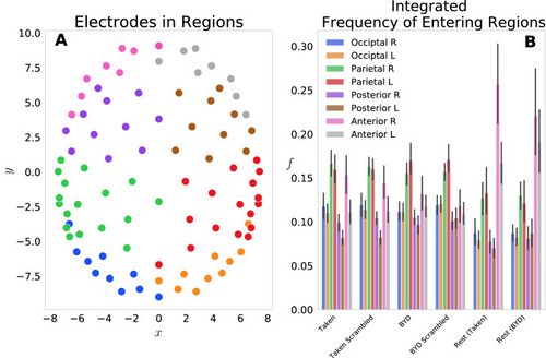
Figure 1 : (A) Emplacements des électrodes pour chacune des 92 électrodes sur le capuchon de tête de Electrical Geodesics Inc. Les électrodes ont été projetées sur un plan horizontal avec le nez dans la direction y positive. Les électrodes ont été codées par couleur pour afficher les éléments constitutifs des 8 groupes pour l'analyse de fréquence, à savoir, occipital gauche (bleu)/droit (orange), pariétal gauche (vert)/droit (rouge), postérieur gauche (violet)/ droite (marron) et antérieure gauche (rose)/droite (gris).
(B) Des histogrammes représentant la fréquence d'entrée dans chaque région fG sont affichés pour les six conditions testées. Un changement significatif dans le stimulus est présent entre chacune des régions antérieures gauche et droite lors de la comparaison du repos pré-stimulus et de l'état stimulé respectif (P < 0,001, Tukey ajusté.). Les barres d'erreur affichent l'intervalle de confiance de 1 écart type.
Espace des phases
Nous avons également exploré l'espace des phases de valeur moyenne de ce système. L'espace de phase pour chaque sujet a été tracé comme la position et l'impulsion moyennes le long de la direction ,  ou comme la position et l'impulsion moyennes le long de la direction ,
  . La figure 2 montre les centroïdes des diagrammes de dispersion de l'espace de phase pour chaque sujet avec une ellipse représentant l'intervalle de confiance à un écart-type. Notez que les valeurs ne sont rapportées que pour les stimuli intacts car une analyse de la variance montre que les films brouillés et intacts ne se distinguent pas dans l'espace des phases (
 , Tukey ajusté).
Les figures 2A et B montrent la projection du centroïde de l'espace des phases sur le plan enjambé par et  pour "Bang ! You're Dead » et « Taken » respectivement, et le plan Fig. 2C et D (
 ). La position moyenne le long de l'axe ,
  pour le stimulus intact (« BYD » et « Prise ») et leurs formes brouillées sont significativement différentes des homologues de repos pré-stimulus avec (ajustement de Tukey) alors que les centroïdes positifs à la tâche et au repos sont indiscernable dans le plan (
  , Tukey ajusté).
Les moyennes du groupe sont rapportées dans le tableau 11 avec leurs écarts-types. Ces valeurs sont la valeur moyenne des centroïdes (moyenne des points centraux des stimuli sur la figure 2) pour la position/le moment respectif dans chaque niveau de stimulus. Comme on le voit également sur les figures 2C et D, il existe une différence frappante d'un ordre de grandeur pour  entre les conditions de repos et de tâche, mais aucune différence marquée ,
  dans
dans  .
.
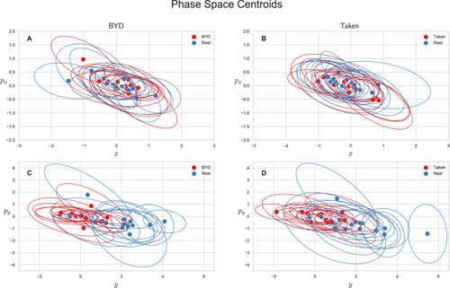
Figure 2 : Centroïdes moyens de l'espace de phase pour chaque sujet. Les ellipses représentent l'intervalle de confiance à 1 écart type. Les centroïdes des stimuli brouillés ont été omis car ils ne peuvent pas être distingués des stimuli intacts (P > 0,85)
(A) Centroïdes pour "Bang ! Tu es mort » le long de la direction x.
(B) Centroïdes pour "Prise" le long de la direction x.
(C) Centroïdes pour "Bang ! Tu es mort » dans la direction y.
(D) Centroïdes pour "Prise" le long de la direction y. Les différences ne sont apparentes que dans la direction y (P < 0,001, ajusté de Tukey) indiquant le niveau plus élevé d'activation antérieure comme indiqué sur la Fig. 1.
Tableau 1
Moyennes de groupe des centroïdes.
| Stimulus
|

|
|
|
|
| Pris
|

|

|

|

|
| Prise brouillée
|

|

|

|

|
| Claquer! Tu es mort
|

|

|

|

|
| Claquer! Vous êtes mort brouillé
|

|

|

|

|
| Repos (pré-pris)
|

|

|

|

|
| Repos (pré-BYD)
|

|

|

|

|
Des différences significatives ne sont notées que pour le reste acquis avant Taken et Bang ! Vous êtes mort lorsque vous comparez l'emplacement y moyen à l'un de leurs homologues de tâche (stimulus brouillés et intacts).
Moyennes de groupe des centroïdes.
Cette analyse a révélé deux résultats notables. Premièrement, il y avait un manque de différences significatives dans les impulsions du cerveau le long de la direction x et y. Deuxièmement, les moyennes des impulsions n'étaient pas significativement différentes de 0 au niveau du groupe. Les impulsions positives ou négatives proviennent de la dérivée temporelle concurrente de la probabilité et de l'emplacement de l'électrode. Puisque la moyenne des moments est de 0, il y a un nombre égal d'électrodes antérieures et postérieures avec à la fois des augmentations et des diminutions de probabilité.
De plus, nous avons examiné les changements dans les valeurs de probabilité dans les états de repos et d'activité. Des animations des distributions de probabilité sont présentes dans le matériel supplémentaire 1. Dans ces animations, les différences de repos et de tâche sont apparentes à travers l'évolution de la probabilité dans le temps.
Principe incertain.
Malgré la confirmation des résultats neuroscientifiques antérieurs et le succès apparent de notre modèle quasi-quantique, notre question de recherche telle que posée ci-dessus ne reste qu'à moitié résolue. En utilisant ce modèle, nous avons noté des différences dans les distributions de probabilité et les centroïdes de l'espace des phases au repos par rapport à la tâche. Cependant, nous cherchions toujours un paramètre du modèle qui resterait le même en repos et en tâche. À cette fin, nous avons défini un principe d'incertitude de Heisenberg analogue de la forme,
|
|

|

|
Le tableau 2 affiche les valeurs de cette constante () acquises dans toutes les conditions, ainsi que la valeur maximale, la valeur moyenne et l'écart type. Nous avons constaté que ce modèle quasi-quantique conduit à une valeur minimale constante entre  et
et  de
de  avec
avec  .
.
Notez que l'unité de  est le résultat de l'EEG échantillonné à 250 Hz et que la masse est considérée comme l'unité. De plus, la valeur moyenne et l'écart type de ces quantités restent cohérents dans toutes les conditions avec une valeur moyenne de
  ( ) et un écart type de
  ().
().
Notamment, la valeur maximale varie entre les conditions, la valeur la plus élevée se produisant lorsque les sujets regardaient le clip intact de Bang ! Tu es mort. Bien que la position moyenne du signal le long de la direction y soit différente au repos que pendant une tâche (), la méthodologie mathématique quasi-quantique conduit à une valeur d'incertitude constante.
De manière assez remarquable, les valeurs du tableau montrent que l'incertitude moyenne et l'incertitude minimale sont les mêmes dans différentes conditions, malgré des maxima variant de plus de deux ordres de grandeur. Ainsi, donner plus de crédibilité à l'idée que cette relation d'incertitude capture les similitudes du cerveau dans des conditions très différentes. La figure 3 affiche la distribution de probabilité au moment correspondant au minimum d'incertitude pour et .
Table 2
Différentes valeurs extraites des évolutions temporelles des produits
and .
| Stimulus
|

|

|
|
|
|
|
|
|
| Pris
|

|

|

|

|

|
|

|

|
| Prise brouillée
|

|

|

|

|

|

|
|

|
| Claquer! Tu es mort
|

|

|

|

|

|

|

|

|
| Claquer! Vous êtes mort brouillé
|

|

|

|

|

|

|

|

|
| Repos (pré-pris)
|

|

|

|

|

|
|
|

|
| Repos (pré-BYD)
|

|

|

|

|

|

|

|

|
Considérant la valeur minimale que ces produits atteignent pour chaque sujet, nous voyons une valeur constante en x et y de , une valeur moyenne de et un écart type constant de . L'unité de provient de l'échantillonnage de 250 Hz. Les valeurs maximales diffèrent selon la stimulation. Les valeurs sont rapportées sous forme de moyenne entre les sujets plus ou moins 1 écart type.
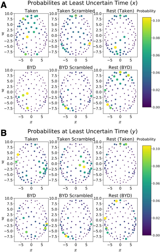
Figure 3: Cartes de probabilité correspondant au point temporel le moins incertain pour chacune des six conditions expérimentales.
(A) Les probabilités qui conduisent à l'incertitude minimale telle que définie par le minimum de
.
(B) Les probabilités qui conduisent à l'incertitude minimale telle que définie par le minimum de
. Un sujet est affiché pour tous les stimuli pris, et un autre pour tous les stimuli Bang ! Vous êtes des stimuli morts.
Discussion
Dans la présente étude, nous avons étudié l'étendue spatiale et les propriétés transitoires associées de l'activité neuronale dans le cerveau pendant les conditions actives et de repos, et si des propriétés de réseau sous-jacentes similaires existent. Nous avons constaté que l'application de la transformation de Hilbert aux données EEG et sa normalisation (Eq. 2) impose une structure probabiliste au signal EEG à travers le cerveau (Eq. 3), que nous avons utilisée pour identifier la probabilité des modèles spatiaux d'activité ainsi que les transitions en activité sur tout le cuir chevelu. Nous avons trouvé plus d'activité antérieure pendant le repos par rapport à l'observation du film, à la fois dans l'amplitude et dans l'espace de phase. Cette constatation est conforme aux résultats précédents montrant une activation accrue dans la région antérieure pendant le repos.[21][21][22][34][37][38] De plus, en normalisant les signaux EEG transformés de Hilbert et en extrayant des valeurs moyennes similaires à celles de la formulation de la fonction d'onde de la mécanique quantique, nous avons pu calculer l'incertitude de la «position» et de la «momentum» pendant le repos et le visionnage de films, qui est définie par la nouvelle constante 
Il est séduisant d'associer la constante liée à la «position» et à la «momentum» de l'activité neuronale à un principe fondamental, tel que le principe d'incertitude de Heisenberg. Cependant, on ne sait toujours pas ce que signifie cette incertitude. Cela pourrait impliquer des limites au degré auquel le cerveau est accessible ; l'augmentation des informations sur l'emplacement précis de l'état du cerveau (tel que décrit par nos «fonctions d'onde» quasi-quantiques) produira une plus grande incertitude quant à l'endroit où il se trouvera à un moment ultérieur. Ces résultats offrent une perspective intéressante sur le lien entre la fonction neuronale et les processus cognitifs. Par exemple, à mesure que la "fonction d'onde" se localise dans l'espace le long d'un train de pensées, nous devenons distraits pour augmenter l'incertitude, ce qui peut expliquer pourquoi les esprits errent et les pensées sont éphémères ?
La valeur  que nous avons trouvée est-elle constante dans différentes conditions de stimulation et indépendante du nombre d'électrodes utilisées pour acquérir les données ? Pour tester cela, nous avons échantillonné les électrodes EEG de 92 à 20 et effectué la même analyse que dans le texte principal. Conformément aux 92 canaux, nous avons trouvé la tendance antérieure au repos, mais nous avons constaté que la réduction des électrodes à 20 entraînait une constante différente
  (voir le matériel supplémentaire).
Cela démontre que le modèle est capable de capturer les différences de repos/tâche, mais une condition de normalisation dépendante du montage peut devoir être introduite.
Il est important de noter que les valeurs d'incertitude de cette forme sont inhérentes à toute variable conjuguée de Fourier, car une valeur s'étale dans une variable, elle se localise dans l'autre. Cela suggère qu'après avoir défini le carré de l'évolution temporelle de l'électrode EEG transformée de Hilbert comme étant la probabilité et imposé les propriétés d'un espace de Hilbert sur les signaux d'électrode, une valeur d'incertitude peut être extraite. En mécanique quantique, cette incertitude fixe la limite des échelles non observables. Cette approche a été inspirée par le besoin en neurosciences de nouveaux modèles pour aider à interpréter les données de neuroimagerie. Bien qu'il s'agisse d'une avancée méthodologique intéressante, nous devons encore déterminer si l'incertitude observée dans les données EEG est soutenue par un nouveau principe fondamental comme en mécanique quantique, ou si c'est simplement le résultat d'avoir construit deux nouvelles variables conjuguées de Fourier à partir du Signal EEG.
Des travaux supplémentaires doivent être effectués pour explorer cette constante en ce qui concerne la riche taxonomie des tâches et des stimuli et les différents états de conscience qui sont couramment utilisés en neurosciences cognitives. Cette méthodologie pourrait être étendue à l'IRMf, où les cours temporels BOLD pourraient être transformés par Hilbert, créant ainsi un analogue tridimensionnel du modèle EEG présenté dans cet article.
En fin de compte, cet article a présenté une nouvelle méthodologie pour analyser les données EEG. Normaliser les données et les traiter comme une amplitude de probabilité a conduit à des paramètres qui changeaient avec la présence ou l'absence de stimulus, tout en établissant simultanément une valeur constante indépendante du stimulus. Nous avons appliqué avec succès un cadre mathématique basé sur les formalismes de la mécanique quantique au paradigme du repos et de la tâche en EEG (sans prétendre que le cerveau est un objet quantique). Alors que les neurosciences continuent d'évoluer, les outils analytiques à leur disposition doivent également progresser en conséquence. Nous espérons que cet outil analytique, ainsi que les progrès de la modélisation et de l'apprentissage automatique, nous aideront à comprendre la nature de la conscience.
Méthodes
L'acquisition des données
Vingt-huit sujets sains ont été recrutés au Brain and Mind Institute de l'Université de Western Ontario, au Canada, pour participer à cette étude. Un consentement écrit éclairé a été obtenu avant le test de tous les participants. L'approbation éthique de cette étude a été accordée par le comité d'éthique de la recherche en sciences de la santé et le comité d'éthique de la recherche non médicale de l'Université de Western Ontario et toutes les recherches ont été effectuées conformément aux lignes directrices/règlements pertinents et conformément à la Déclaration d'Helsinki.
Deux extraits de films pleins de suspense ont été utilisés comme stimuli naturalistes dans cette étude. Un extrait vidéo du film muet « Bang ! You're Dead" et un extrait audio du film "Taken" ont été montrés à 13 et 15 sujets respectivement dans leurs formes originales intactes et brouillées. Avant les deux acquisitions, une section de repos a été acquise où les sujets ont été invités à se détendre, sans aucune stimulation manifeste. La présentation du stimulus a été contrôlée avec le plugin Psychtoolbox pour MATLAB[39][40][41] sur un Apple MacBook Pro 15″. L'audio a été présenté de manière binaurale à un volume d'écoute confortable via les écouteurs Etymotics ER-1.
Les données EEG ont été recueillies à l'aide d'un capuchon à 129 canaux (Electrical Geodesics Inc. [EGI], Oregon, États-Unis). Les impédances des électrodes ont été maintenues en dessous de 50 kΩ avec des signaux échantillonnés à 250 Hz et référencés au sommet central (Cz). À l'aide de la boîte à outils EEGLAB MATLAB,[42] les canaux bruyants ont été identifiés et supprimés, puis réinterpolés dans les données. Un test de Kolmogorov-Smirnov (KS) sur les données a été utilisé pour identifier les régions qui n'étaient pas gaussiennes. L'analyse des composants indépendants (ICA) a ensuite été utilisée pour identifier visuellement les modèles d'activité neuronale caractéristiques des mouvements oculaires et musculaires qui ont ensuite été supprimés des données. Le prétraitement EEG a été effectué individuellement pour chaque sujet et condition.
Parmi les deux extraits de films testés, le premier était un segment de 8 minutes du film muet télévisé d'Alfred Hitchcock "Bang ! Tu es mort". Cette scène met en scène un garçon de 5 ans qui ramasse le revolver de son oncle. Le garçon charge une balle dans le pistolet et joue avec comme s'il s'agissait d'un jouet. Le garçon (et le spectateur) sait rarement si l'arme a une balle dans sa chambre et le suspense monte lorsque le garçon fait tourner la chambre, la pointe vers les autres et appuie sur la gâchette. Comme alternative à la stimulation visuelle, un extrait audio de 5 minutes du film "Taken" a également été utilisé. Ce clip dépeint une conversation téléphonique dans laquelle un père surprend l'enlèvement de ses filles.
De plus, deux stimuli de contrôle « brouillés » ont été utilisés, un pour chaque film. Cela sépare les réponses neuronales suscitées par les propriétés sensorielles de regarder ou d'écouter les films de celles impliquées dans le suivi de l'intrigue. La version brouillée de "Bang ! You're Dead » a été généré en isolant les segments de 1 s et en mélangeant les segments de manière pseudo-aléatoire, éliminant ainsi la cohérence temporelle du récit.[43] La version brouillée de "Taken" a été créée en faisant tourner spectralement l'audio, rendant ainsi le discours indéchiffrable.[43][44] Les extraits de films brouillés ont été présentés avant les versions intactes pour éviter les effets de report potentiels du récit. Avant que les sujets regardent/écoutent le stimulus brouillé, un court segment d'EEG au repos a été acquis.
Modèle
Chacune des j électrodes est décrite par un couple ordonné ( ) dans un espace tridimensionnel. Pour compléter cette analyse, les électrodes ont d'abord été projetées sur le plan (
 ) en supprimant la profondeur de la tête. La figure 1A montre les emplacements de chaque électrode dans cet espace 2d. Suite à cette projection, les cours du temps pour chacune des 92 électrodes ont été transformés de Hilbert puis normalisés en suivant la procédure indiquée à l'aide de l'Eq. (2). Une probabilité a été définie dans cet espace de position d'électrode comme le carré de l'évolution temporelle de la transformée de Hilbert (Eq. 3), analogue aux fonctions d'onde de la mécanique quantique. Huit régions Antérieure G/D, Postérieure G/D, Pariétale G/D, Occipitale G/D) ont ensuite été définies en regroupant les 92 électrodes, et les fréquences d'entrée dans chaque région fG ont été obtenues en sommant les probabilités des électrodes au sein du groupe, puis intégration dans le temps.
|
|

|

|
où chacun des huit groupes désignés par l'indice a un nombre différent d'électrodes constitutives N. Dans l'occipital gauche et droit il y a 10 électrodes chacun, dans le pariétal gauche et droit il y a 17 électrodes chacun, dans la partie postérieure gauche et droite il y a sont respectivement 10 et 11 électrodes, et dans les parties antérieures gauche et droite, il y a respectivement 8 et 9 électrodes.
Après avoir obtenu les fréquences de niveau de groupe, les valeurs moyennes pour la position et l'élan ont été calculées à l'aide des équations. (4) et (5) (avec des expressions identiques pour y). Enfin, pour vérifier notre principe d'incertitude analogue, nous avons cherché des expressions de la forme
|
|

|

|
L'expression pour peut être facilement appliquée aux probabilités et positions telles que définies ci-dessus, résultant en le premier terme donné par
|
|

|

|
Et le second terme donné par le carré de l'Eq. (4). Le second terme de  est donné par le carré de l'Eq. (5), mais le premier terme est plus nuancé. Cela est dû au nombre complexe renvoyé en agissant deux fois sur l'opérateur dérivé sur la probabilité. Pour surmonter cela, des transformées de Fourier ont été utilisées pour modifier l'équation. (5) dans la base de quantité de mouvement qui a ensuite permis le calcul efficace de
  .
.
En désignant  comme la probabilité impulsion-espace obtenue par une transformée de Fourier bidimensionnelle non uniforme de la pseudo-fonction d'onde de l'espace de position, Eq. (5) peut être réécrit comme,
|
|

|

|
Conduisant au premier terme de l'expression à écrire comme,
|
|
![{\displaystyle \langle p_{x}^{2}(t)\rangle =m^{2}\sum _{j=1}^{92}{\tfrac {x_{j}^{2}}{{\tilde {p}}_{j}(t)}}[{d \over dt}P_{j}(t)]^{2}}](https://wikimedia.org/api/rest_v1/media/math/render/svg/3dda471e5a09b53812126091bf6b9a73fc19a4f4)
|

|
Le wrapper python FINUFFT a été utilisé pour prendre la transformée de Fourier en utilisant une FFT[45][46] non uniforme de type 3, 2d, et la valeur minimale dans le temps de la relation d'incertitude a été trouvée. Des points dans l'espace d'impulsion ont été échantillonnés sur ![{\displaystyle p_{x}\in [-4,4]}](https://wikimedia.org/api/rest_v1/media/math/render/svg/515f4df54a0052df61a308afa0bb41739bf89ef0) et
et ![{\displaystyle p_{y}\in [-4,5]}](https://wikimedia.org/api/rest_v1/media/math/render/svg/950ccba52979e32d86080daf5a94cb3b5524feb6) avec les deux points supplémentaires (
avec les deux points supplémentaires (![{\displaystyle [-5,-4]}](https://wikimedia.org/api/rest_v1/media/math/render/svg/c1acb0cb7df6bce649ff45049f7f85ca28c1c5b7) ) et (
) et (![{\displaystyle [-4,-5]}](https://wikimedia.org/api/rest_v1/media/math/render/svg/c01ceeb13f42e4e0cc0444eefecc2e668333a503) ). La figure 4 montre les probabilités de position et d'impulsion respectivement dans leur propre base. Matériel supplémentaire 2.
). La figure 4 montre les probabilités de position et d'impulsion respectivement dans leur propre base. Matériel supplémentaire 2.
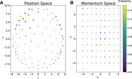
Figure 4: (A) Distribution de probabilité pour un seul sujet dans la base de position. (B) Distribution de probabilité de base de l'élan pour un seul sujet. Les valeurs de quantité de mouvement utilisées pour la transformée de Fourier sont indiquées par les emplacements des points. Les points sont codés par couleur/taille pour représenter la valeur de probabilité à cet emplacement. Pour calculer les valeurs rapportées dans le tableau 2, la valeur correspondante a été trouvée pour chaque sujet, et celles-ci ont été utilisées pour calculer la moyenne du groupe rapportée ici.
Information supplémentaire
Figures supplémentaires.(28M, docx)
Informations supplémentaires.(375K, docx)
Remerciements
Nous tenons à remercier Silvano Petrarca pour son aide continue dans la conception du modèle. Cette étude a été financée par la Subvention à la découverte du CRSNG (05578-2014RGPIN), CERC (215063), Fonds de la Fondation des CIHR (167264). AMO est Fellow du programme Cerveau, esprit et conscience de l'CIFAR.
Contributions d'auteur
N.J.M.P., C.M. et G.L. ont effectué l'analyse. A.S., B.S. et N.J.M.P. développé le modèle. COMME. et BS supervisé l'analyse. N.J.M.P., A.S., G.L. et B.S. écrit le manuscrit. A.M.O. révisé le manuscrit.
Intérêts concurrents
Les auteurs ne déclarent aucun intérêt concurrent.
Notes de bas de page
Note de l'éditeur
Springer Nature reste neutre en ce qui concerne les revendications juridictionnelles dans les cartes publiées et les affiliations institutionnelles.
Ces auteurs ont contribué à parts égales : Bobby Stojanoski et Andrea Soddu.
Information supplémentaire
La version en ligne contient du matériel supplémentaire disponible au 10.1038/s41598-021-97960-7.
Informations sur l'article
Sci Rep. 2021; 11: 19771.
Published online 2021 Oct 5. doi: 10.1038/s41598-021-97960-7
PMCID: PMC8492705
PMID: 34611185
Nicholas J. M. Popiel,1,2 Colin Metrow,1 Geoffrey Laforge,3 Adrian M. Owen,3,4,5 Bobby Stojanoski,#4,6 and Andrea Soddu#1,3
1The Department of Physics and Astronomy, The University of Western Ontario, London, ON N6A 5B7 Canada
2Cavendish Laboratory, University of Cambridge, Cambridge, CB3 0HE UK
3The Brain and Mind Institute, The University of Western Ontario, London, ON N6A 5B7 Canada
4The Department of Psychology, The University of Western Ontario, London, ON N6A 5B7 Canada
5The Department of Physiology and Pharmacology, The University of Western Ontario, London, ON N6A 5B7 Canada
6Faculty of Social Science and Humanities, University of Ontario Institute of Technology, 2000 Simcoe Street North, Oshawa, ON L1H 7K4 Canada
Andrea Soddu, Email: asoddu@uwo.ca
Corresponding author.
- Contributed equally.
Received 2021 Apr 28; Accepted 2021 Aug 30.
Copyright © The Author(s) 2021
Libre accès
Cet article est sous licence Creative Commons Attribution 4.0 International, qui autorise l'utilisation, le partage, l'adaptation, la distribution et la reproduction sur tout support ou format, tant que vous donnez le crédit approprié à l'auteur ou aux auteurs originaux et à la source, fournissez un lien vers la licence Creative Commons, et indiquez si des modifications ont été apportées. Les images ou tout autre matériel de tiers dans cet article sont inclus dans la licence Creative Commons de l'article, sauf indication contraire dans une ligne de crédit au matériel. Si le matériel n'est pas inclus dans la licence Creative Commons de l'article et que votre utilisation prévue n'est pas autorisée par la réglementation légale ou dépasse l'utilisation autorisée, vous devrez obtenir l'autorisation directement du détenteur des droits d'auteur. Pour voir une copie de cette licence, visitez http://creativecommons.org/licenses/by/4.0/.
Les articles des rapports scientifiques sont fournis ici avec l'aimable autorisation de == Nature Publishing Group ==
Bibliography & references
- ↑ Biswal B, Zerrin Yetkin F, Haughton VM, Hyde JS, «Functional connectivity in the motor cortex of resting human brain using echo-planar MRI», in Magn Reson Med, 1995».
PMID:8524021
DOI:10.1002/mrm.1910340409
- ↑ Hutchison RM, Womelsdorfb T, Allenc EA, Bandettini PA, Calhound VD, Corbetta M, Della Penna S, «Dynamic functional connectivity: Promise, issues, and interpretations», in Neuroimage, 2013».
PMID:23707587 - PMCID:PMC3807588
DOI:10.1016/j.neuroimage.2013.05.079
- ↑ Eickhoff SB, Yeo BTT, Genon S, «Imaging-based parcellations of the human brain», in Nat Rev Neurosci, 2018».
PMID:30305712
DOI:10.1038/s41583-018-0071-7
- ↑ Dajani DR, Burrows CA, Odriozola P, Baez A, Nebel MB, Mostofsky SH, Uddin LQ, «Investigating functional brain network integrity using a traditional and novel categorical scheme for neurodevelopmental disorders», in NeuroImage Clin, 2019».
PMID:30708240 - PMCID:PMC6356009
DOI:10.1016/j.nicl.2019.101678
- ↑ Uddin LQ, Karlsgodt KH, «Future directions for examination of brain networks in neurodevelopmental disorders», in J Clin Child Adolesc Psychol, Society of Clinical Child & Adolescent Psychology, 2018».
PMID:29634380 - PMCID:PMC6842321
DOI:10.1080/15374416.2018.1443461
- ↑ Sripada C, Rutherford S, Angstadt M, Thompson WK, Luciana M, Weigard A, Hyde LH, «Prediction of neurocognition in youth from resting state fMRI», in Mol Psychiatry, 2020».
PMID:31427753 - PMCID:PMC7055722
DOI:10.1038/s41380-019-0481-6
- ↑ Biswal BB, Eldreth DA, Motes MA, Rypma B. Task-dependent individual differences in prefrontal connectivity. Cereb. Cortex. 2010;20:2188–2197. doi: 10.1093/cercor/bhp284. [PMC free article][PubMed] [CrossRef] [Google Scholar]
- ↑ Fox MD, Raichle ME. Spontaneous fluctuations in brain activity observed with functional magnetic resonance imaging. Nat. Rev. Neurosci. 2007;8:700–711. doi: 10.1038/nrn2201. [PubMed] [CrossRef] [Google Scholar]
- ↑ Kraus BT, et al. Network variants are similar between task and rest states. Neuroimage. 2021;229:117743. doi: 10.1016/j.neuroimage.2021.117743. [PMC free article][PubMed] [CrossRef] [Google Scholar]
- ↑ Kristo G, et al. Task and task-free FMRI reproducibility comparison for motor network identification. Hum. Brain Mapp. 2014;35:340–352. doi: 10.1002/hbm.22180. [PMC free article][PubMed] [CrossRef] [Google Scholar]
- ↑ Sui J, Adali T, Pearlson GD, Calhoun VD. An ICA-based method for the identification of optimal FMRI features and components using combined group-discriminative techniques. Neuroimage. 2009;46:73–86. doi: 10.1016/j.neuroimage.2009.01.026.[PMC free article] [PubMed] [CrossRef] [Google Scholar]
- ↑ Calhoun VD, Kiehl KA, Pearlson GD. Modulation of temporally coherent brain networks estimated using ICA at rest and during cognitive tasks. Hum. Brain Mapp. 2008;29:828–838. doi: 10.1002/hbm.20581. [PMC free article] [PubMed] [CrossRef] [Google Scholar]
- ↑ Xie H, et al. Whole-brain connectivity dynamics reflect both task-specific and individual-specific modulation: A multitask study. Neuroimage. 2018;180:495–504. doi: 10.1016/j.neuroimage.2017.05.050. [PMC free article] [PubMed] [CrossRef] [Google Scholar]
- ↑ Naci L, Cusack R, Anello M, Owen AM. A common neural code for similar conscious experiences in different individuals. Proc. Natl. Acad. Sci. U. S. A. 2014;111:14277–14282. doi: 10.1073/pnas.1407007111. [PMC free article] [PubMed] [CrossRef] [Google Scholar]
- ↑ Kannurpatti SS, Rypma B, Biswal BB. Prediction of task-related BOLD fMRI with amplitude signatures of resting-state fMRI. Front. Syst. Neurosci. 2012;6:7. doi: 10.3389/fnsys.2012.00007.[PMC free article] [PubMed] [CrossRef] [Google Scholar]
- ↑ Elliott ML, et al. General functional connectivity: Shared features of resting-state and task fMRI drive reliable and heritable individual differences in functional brain networks. Neuroimage. 2019;189:516–532. doi: 10.1016/j.neuroimage.2019.01.068. [PMC free article][PubMed] [CrossRef] [Google Scholar]
- ↑ Cole MW, Ito T, Cocuzza C, Sanchez-Romero R. The functional relevance of task-state functional connectivity. J. Neurosci. 2021 doi: 10.1523/JNEUROSCI.1713-20.2021. [PMC free article][PubMed] [CrossRef] [Google Scholar]
- ↑ Zhang S, et al. Characterizing and differentiating task-based and resting state fMRI signals via two-stage sparse representations. Brain Imaging Behav. 2016;10:21–32. doi: 10.1007/s11682-015-9359-7.[PMC free article] [PubMed] [CrossRef] [Google Scholar]
- ↑ Monier C, Chavane F, Baudot P, Graham LJ, Frégnac Y. Orientation and direction selectivity of synaptic inputs in visual cortical neurons: A diversity of combinations produces spike tuning. Neuron. 2003;37:663–680. doi: 10.1016/S0896-6273(03)00064-3.[PubMed] [CrossRef] [Google Scholar]
- ↑ Churchland MM, et al. Stimulus onset quenches neural variability: A widespread cortical phenomenon. Nat. Neurosci. 2010;13:369–378. doi: 10.1038/nn.2501. [PMC free article][PubMed] [CrossRef] [Google Scholar]
- ↑ 21.0 21.1 21.2 He BJ. Spontaneous and task-evoked brain activity negatively interact. J. Neurosci. 2013;33:4672–4682. doi: 10.1523/JNEUROSCI.2922-12.2013. [PMC free article][PubMed] [CrossRef] [Google Scholar]
- ↑ 22.0 22.1 22.2 Bonnard M, et al. Resting state brain dynamics and its transients: A combined TMS-EEG study. Sci. Rep. 2016;6:1–9. doi: 10.1038/srep31220. [PMC free article] [PubMed] [CrossRef] [Google Scholar]
- ↑ 23.0 23.1 Axelrod V, Zhu X, Qiu J. Transcranial stimulation of the frontal lobes increases propensity of mind-wandering without changing meta-awareness. Sci. Rep. 2018;8:1–14. doi: 10.1038/s41598-018-34098-z. [PMC free article] [PubMed] [CrossRef] [Google Scholar]
- ↑ 24.0 24.1 24.2 Axelrod V, Rees G, Lavidor M, Bar M. Increasing propensity to mind-wander with transcranial direct current stimulation. Proc. Natl. Acad. Sci. U. S. A. 2015;112:3314–3319. doi: 10.1073/pnas.1421435112. [PMC free article] [PubMed] [CrossRef] [Google Scholar]
- ↑ 25.0 25.1 Townsend JS. A Modern Approach to Quantum Mechanics.University Science Books; 2012. [Google Scholar]
- ↑ Heisenberg W. Über den anschaulichen Inhalt der quantentheoretischen Kinematik und Mechanik. Z. Phys. 1927;43:172–198. doi: 10.1007/BF01397280. [CrossRef] [Google Scholar]
- ↑ Penrose R. The Emperor’s New Mind. Viking Penguin; 1990. [Google Scholar]
- ↑ Penrose R. Shadows of the Mind: A Search for the Missing Science of Consciousness. Oxford University Press; 1994. [Google Scholar]
- ↑ Atmanspacher H. Quantum Approaches to Consciousness.Stanford Encyclopedia of Philosophy; 2004. [Google Scholar]
- ↑ Hameroff S. How quantum brain biology can rescue conscious free will. Front. Integr. Neurosci. 2012;6:93. doi: 10.3389/fnint.2012.00093. [PMC free article] [PubMed] [CrossRef] [Google Scholar]
- ↑ Freeman WJ, Vitiello G. Nonlinear brain dynamics as macroscopic manifestation of underlying many-body field dynamics. Phys. Life Rev. 2006;3:93–118. doi: 10.1016/j.plrev.2006.02.001.[CrossRef] [Google Scholar]
- ↑ le Van Quyen M, et al. Comparison of Hilbert transform and wavelet methods for the analysis of neuronal synchrony. J. Neurosci. Methods. 2001;111:83–98. doi: 10.1016/S0165-0270(01)00372-7.[PubMed] [CrossRef] [Google Scholar]
- ↑ Freeman WJ. Deep analysis of perception through dynamic structures that emerge in cortical activity from self-regulated noise. Cogn. Neurodyn. 2009;3:105–116. doi: 10.1007/s11571-009-9075-3.[PMC free article] [PubMed] [CrossRef] [Google Scholar]
- ↑ 34.0 34.1 Wang RWY, Chang WL, Chuang SW, Liu IN. Posterior cingulate cortex can be a regulatory modulator of the default mode network in task-negative state. Sci. Rep. 2019;9:1–12. [PMC free article][PubMed] [Google Scholar]
- ↑ Uddin LQ, Kelly AMC, Biswal BB, Castellanos FX, Milham MP. Functional connectivity of default mode network components: Correlation, anticorrelation, and causality. Hum. Brain Mapp. 2009;30:625–637. doi: 10.1002/hbm.20531. [PMC free article][PubMed] [CrossRef] [Google Scholar]
- ↑ Stawarczyk D, Majerus S, Maquet P, D’Argembeau A. Neural correlates of ongoing conscious experience: Both task-unrelatedness and stimulus-independence are related to default network activity. PLoS One. 2011;6:e16997. doi: 10.1371/journal.pone.0016997.[PMC free article] [PubMed] [CrossRef] [Google Scholar]
- ↑ 37.0 37.1 Greicius, M. D., Krasnow, B., Reiss, A. L., Menon, V. & Raichle, M. E. Functional Connectivity in the Resting Brain: A Network Analysis of the Default Mode Hypothesis. www.pnas.org. [PMC free article] [PubMed]
- ↑ Christoff K, Gordon AM, Smallwood J, Smith R, Schooler JW. Experience sampling during fMRI reveals default network and executive system contributions to mind wandering. Proc. Natl. Acad. Sci. U. S. A. 2009;106:8719–8724. doi: 10.1073/pnas.0900234106.[PMC free article] [PubMed] [CrossRef] [Google Scholar]
- ↑ Brainard DH. The psychophysics toolbox. Spat. Vis. 1997;10:433–436. doi: 10.1163/156856897X00357. [PubMed] [CrossRef] [Google Scholar]
- ↑ Kleiner M, et al. What’s new in psychtoolbox-3. Perception. 2007;36:1–16. [Google Scholar]
- ↑ Pelli DG. The VideoToolbox software for visual psychophysics: Transforming numbers into movies. Spat. Vis. 1997;10:437–442. doi: 10.1163/156856897X00366. [PubMed] [CrossRef] [Google Scholar]
- ↑ Makeig, S. & Onton, J. ERP features and EEG dynamics: An ICA perspective. In The Oxford Handbook of Event-Related Potential Components (Oxford University Press, 2012). 10.1093/oxfordhb/9780195374148.013.0035.
- ↑ 43.0 43.1 Laforge G, Gonzalez-Lara LE, Owen AM, Stojanoski B. Individualized assessment of residual cognition in patients with disorders of consciousness. NeuroImage Clin. 2020;28:102472. doi: 10.1016/j.nicl.2020.102472. [PMC free article] [PubMed] [CrossRef] [Google Scholar]
- ↑ Naci L, Sinai L, Owen AM. Detecting and interpreting conscious experiences in behaviorally non-responsive patients. Neuroimage. 2017;145:304–313. doi: 10.1016/j.neuroimage.2015.11.059.[PubMed] [CrossRef] [Google Scholar]
- ↑ Barnett AH, Magland J, Klinteberg LAF. A parallel nonuniform fast Fourier transform library based on an “Exponential of semicircle” kernel. SIAM J. Sci. Comput. 2019;41:C479–C504. doi: 10.1137/18M120885X. [CrossRef] [Google Scholar]
- ↑ Barnett, A. H. Aliasing error of the kernel in the nonuniform fast Fourier transform. arXiv:2001.09405 [math.NA] (2020).
Masticationpedia is a charity, a not-for-profit organization operating in dentistry medical research,
particularly focusing on the field of the neurophysiology of the masticatory system


