|
|
| Line 1: |
Line 1: |
| {{transl}} | | {{transl|de}} |
|
| |
|
| {{FR | | {{FR |
| Line 40: |
Line 40: |
| {{Bookind2}} | | {{Bookind2}} |
|
| |
|
| == Abstract==
| | {{:Store:EEMIde01}} |
|
| |
|
| An outstanding issue in cognitive neuroscience concerns how the brain is organized across different conditions. For instance, during the resting-state condition, the brain can be clustered into reliable and reproducible networks (e.g., sensory, default, executive networks). Interestingly, the same networks emerge during active conditions in response to various tasks. If similar patterns of neural activity have been found across diverse conditions, and therefore, different underlying processes and experiences of the environment, is the brain organized by a fundamental organizational principle? To test this, we applied mathematical formalisms borrowed from quantum mechanisms to model electroencephalogram (EEG) data. We uncovered a tendency for EEG signals to be localized in anterior regions of the brain during “rest”, and more uniformly distributed while engaged in a task (i.e., watching a movie). Moreover, we found analogous values to the Heisenberg uncertainty principle, suggesting a common underlying architecture of human brain activity in resting and task conditions. This underlying architecture manifests itself in the novel constant <math>K_{brain}</math>, which is extracted from the brain state with the least uncertainty. We would like to state that we are using the mathematics of quantum mechanics, but not claiming that the brain behaves as a quantum object.
| | {{:Store:EEMIde02}} |
|
| |
|
| | {{:Store:EEMIde03}} |
|
| |
|
| Subject terms: Computational science, Quantum mechanics
| | {{:Store:EEMIde04}} |
|
| |
|
| === Introduction ===
| | {{:Store:EEMIde05}} |
| An important but outstanding issue in contemporary cognitive neuroscience is understanding the organizational properties of neural activity. For instance, is there a fundamental structure to the spatial–temporal patterns neural brain activity across different conditions? One common approach used to address this question is to examine the brain at “rest”. Measures such as functional connectivity, independent component analysis and graph theoretic metrics, have been applied to data recorded using different imaging techniques (e.g., functional magnetic resonance imaging (fMRI) and electroencephalography (EEG)), to cluster brain areas that exhibit similar activity patterns. Numerous studies have shown that brain activity during “rest” can be grouped into distinct networks across<ref>Biswal, B., Zerrin Yetkin, F., Haughton, V. M. & Hyde, J. S. Functional connectivity in the motor cortex of resting human brain using echo-planar MRI. Magn. Reson. Med. 34, 537–541 (1995).</ref><ref>Hutchison,R.M.etal. Dynamic functional connectivity: Promise, issues, and interpretations. Neuroimage80,360–378(2013).</ref>; such as sensory (visual and auditory), default mode, executive, salience, and attentional (ventral and dorsal) networks that have been reliably reproduced across thousands of participants<ref>Eickhoff,S.B.,Yeo,B.T.T.&Genon,S.Imaging-basedparcellationsofthehumanbrain.Nat.Rev.Neurosci.19,672–686(2018).</ref>, and are predictive of phenotypic measures like cognition and clinical diagnoses<ref>Dajani DR, et al. Investigating functional brain network integrity using a traditional and novel categorical scheme for neurodevelopmental disorders. NeuroImage Clin. 2019;21:101678. doi: 10.1016/j.nicl.2019.101678. [PMC free article] [PubMed] [CrossRef] [Google Scholar]</ref><ref>Uddin LQ, Karlsgodt KH. Future directions for examination of brain networks in neurodevelopmental disorders. J. Clin. Child Adolesc. Psychol. 2018;47:483–497. doi: 10.1080/15374416.2018.1443461. [PMC free article] [PubMed] [CrossRef] [Google Scholar]</ref><ref>Sripada C, et al. Prediction of neurocognition in youth from resting state fMRI. Mol. Psychiatry. 2020;25:3413–3421. doi: 10.1038/s41380-019-0481-6. [PMC free article] [PubMed] [CrossRef] [Google Scholar]</ref>. These results suggest these networks may be an intrinsic aspect of neural activity.
| |
|
| |
|
| Indeed, the same set of structured patterns of neural activity have been found during "active" states, such as, while completing different tasks<ref>Biswal BB, Eldreth DA, Motes MA, Rypma B. Task-dependent individual differences in prefrontal connectivity. Cereb. Cortex. 2010;20:2188–2197. doi: 10.1093/cercor/bhp284. [PMC free article][PubMed] [CrossRef] [Google Scholar]</ref><ref>Fox MD, Raichle ME. Spontaneous fluctuations in brain activity observed with functional magnetic resonance imaging. Nat. Rev. Neurosci. 2007;8:700–711. doi: 10.1038/nrn2201. [PubMed] [CrossRef] [Google Scholar]</ref><ref>Kraus BT, et al. Network variants are similar between task and rest states. Neuroimage. 2021;229:117743. doi: 10.1016/j.neuroimage.2021.117743. [PMC free article][PubMed] [CrossRef] [Google Scholar]</ref>. For instance, there is a high degree of correspondence between networks extracted during rest and those extracted during tasks measuring sensorimotor<ref>Kristo G, et al. Task and task-free FMRI reproducibility comparison for motor network identification. Hum. Brain Mapp. 2014;35:340–352. doi: 10.1002/hbm.22180. [PMC free article][PubMed] [CrossRef] [Google Scholar]</ref><ref>Sui J, Adali T, Pearlson GD, Calhoun VD. An ICA-based method for the identification of optimal FMRI features and components using combined group-discriminative techniques. Neuroimage. 2009;46:73–86. doi: 10.1016/j.neuroimage.2009.01.026.[PMC free article] [PubMed] [CrossRef] [Google Scholar]</ref> and higher-level cognitive abilities (i.e., working memory)<ref>Calhoun VD, Kiehl KA, Pearlson GD. Modulation of temporally coherent brain networks estimated using ICA at rest and during cognitive tasks. Hum. Brain Mapp. 2008;29:828–838. doi: 10.1002/hbm.20581. [PMC free article] [PubMed] [CrossRef] [Google Scholar]</ref><ref>Xie H, et al. Whole-brain connectivity dynamics reflect both task-specific and individual-specific modulation: A multitask study. Neuroimage. 2018;180:495–504. doi: 10.1016/j.neuroimage.2017.05.050. [PMC free article] [PubMed] [CrossRef] [Google Scholar]</ref>.Even completing a task as complicated as following the plot of a movie elicits the same network architecture as observed in the resting brain<ref name=":0">Naci L, Cusack R, Anello M, Owen AM. A common neural code for similar conscious experiences in different individuals. Proc. Natl. Acad. Sci. U. S. A. 2014;111:14277–14282. doi: 10.1073/pnas.1407007111. [PMC free article] [PubMed] [CrossRef] [Google Scholar]</ref>. The correspondence between task and rest-based networks is so strong that task-based fMRI network activity can be predicted from the resting state<ref>Kannurpatti SS, Rypma B, Biswal BB. Prediction of task-related BOLD fMRI with amplitude signatures of resting-state fMRI. Front. Syst. Neurosci. 2012;6:7. doi: 10.3389/fnsys.2012.00007.[PMC free article] [PubMed] [CrossRef] [Google Scholar]</ref>, and rest-task network pairs can be identified at the individual level<ref>Elliott ML, et al. General functional connectivity: Shared features of resting-state and task fMRI drive reliable and heritable individual differences in functional brain networks. Neuroimage. 2019;189:516–532. doi: 10.1016/j.neuroimage.2019.01.068. [PMC free article][PubMed] [CrossRef] [Google Scholar]</ref>16. Together, these results suggest that rest and task-based patterns of brain activity likely share a similar underlying neural architecture, despite distinct experiences and cognitive processes<ref>Cole MW, Ito T, Cocuzza C, Sanchez-Romero R. The functional relevance of task-state functional connectivity. J. Neurosci. 2021 doi: 10.1523/JNEUROSCI.1713-20.2021. [PMC free article][PubMed] [CrossRef] [Google Scholar]</ref>.
| | {{:Store:EEMIde06}} |
|
| |
|
| There are, however, important differences between the patterns of brain activity elicited during rest and task-based paradigms, and the set of experiences and cognitive processes associated with each<ref>Zhang S, et al. Characterizing and differentiating task-based and resting state fMRI signals via two-stage sparse representations. Brain Imaging Behav. 2016;10:21–32. doi: 10.1007/s11682-015-9359-7.[PMC free article] [PubMed] [CrossRef] [Google Scholar]</ref>. For instance, the presence or absence of a task is accompanied by increases in variability across different scales including neuronal firing rates changes in field potentials<ref>Monier C, Chavane F, Baudot P, Graham LJ, Frégnac Y. Orientation and direction selectivity of synaptic inputs in visual cortical neurons: A diversity of combinations produces spike tuning. Neuron. 2003;37:663–680. doi: 10.1016/S0896-6273(03)00064-3.[PubMed] [CrossRef] [Google Scholar]</ref><ref>Churchland MM, et al. Stimulus onset quenches neural variability: A widespread cortical phenomenon. Nat. Neurosci. 2010;13:369–378. doi: 10.1038/nn.2501. [PMC free article][PubMed] [CrossRef] [Google Scholar]</ref>, variation in fMRI blood oxygen level dependent (BOLD signal)<ref name=":1">He BJ. Spontaneous and task-evoked brain activity negatively interact. J. Neurosci. 2013;33:4672–4682. doi: 10.1523/JNEUROSCI.2922-12.2013. [PMC free article][PubMed] [CrossRef] [Google Scholar]</ref> and in EEG frequency bands<ref name=":2">Bonnard M, et al. Resting state brain dynamics and its transients: A combined TMS-EEG study. Sci. Rep. 2016;6:1–9. doi: 10.1038/srep31220. [PMC free article] [PubMed] [CrossRef] [Google Scholar]</ref> Furthermore, through transcranial direct current stimulation (tDCS) it has been shown that frontal-lobe stimulation increases one’s proclivity to mind wander <ref name=":8">Axelrod V, Zhu X, Qiu J. Transcranial stimulation of the frontal lobes increases propensity of mind-wandering without changing meta-awareness. Sci. Rep. 2018;8:1–14. doi: 10.1038/s41598-018-34098-z. [PMC free article] [PubMed] [CrossRef] [Google Scholar]</ref><ref name=":3">Axelrod V, Rees G, Lavidor M, Bar M. Increasing propensity to mind-wander with transcranial direct current stimulation. Proc. Natl. Acad. Sci. U. S. A. 2015;112:3314–3319. doi: 10.1073/pnas.1421435112. [PMC free article] [PubMed] [CrossRef] [Google Scholar]</ref>. Importantly, these differences are associated with changes in properties of neural activity but not in changes in the underlying neural architecture.
| | {{:Store:EEMIde07}} |
|
| |
|
| Is there a way to identify the shared neural architecture underlying the cognitive processes associated with rest and active states while also quantifying how these processes diverge from that shared architecture of neural activity? In this paper, we applied mathematical methods analogous to those of quantum mechanics, and the concept of phase space to EEG recorded during rest and movie-watching to extract spatial and transitional properties of dynamic neural activity. Quantum mechanics was developed to describe the dynamics of the subatomic world in terms of probability amplitudes and densities of states. Quantum systems (in the Schrodinger formulation of quantum mechanics) are described by wavefunctions which square to a probability distribution leading to the loss of local determinism and the Heisenberg uncertainty principle (for an overview/intro to the subject see<ref name=":7">Townsend JS. A Modern Approach to Quantum Mechanics.University Science Books; 2012. [Google Scholar]</ref>. This uncertainty principle places a fundamental limit on the location and the momentum of a point particle <ref>Heisenberg W. Über den anschaulichen Inhalt der quantentheoretischen Kinematik und Mechanik. Z. Phys. 1927;43:172–198. doi: 10.1007/BF01397280. [CrossRef] [Google Scholar]</ref>. In essence, if the position of a particle is known there is an underlying uncertainty in its momentum (one cannot precisely say how fast it is going) and vice versa. In addition to the adaptation of the wavefunction approach to quantum mechanics in this paper, we also employed a phase space model. Phase space is a widely used tool in the study of dynamical systems, where the positional variables are paired with their conjugate momenta which establishes a multidimensional space that describes all possible configurations of the given system. This space spans the entire range of states that a system can exist in, each point (in this hyper-space) represents a single state of the system. Phase space and its assorted formalisms are a classical concept, and we simply use it as another tool for analysing the EEG data. Herein, the mathematical methods of quantum mechanics are applied to EEG data to extract a proxy to phase space. This quasi-quantum approach naturally generates the concepts of ‘average’ position, ‘average’ momentum and culminates in an analogous Heisenberg uncertainty principle.
| | {{:Store:EEMIde08}} |
|
| |
|
| In this paper, we posit that using mathematical tools drawn from quantum mechanics, an underlying pattern representative of task and resting brain activity can be realised, in which differences across conditions are apparent, but culminates in a task independent constant value. It is important to note that we are not claiming that the brain behaves as a quantum object as some believe<ref>Penrose R. The Emperor’s New Mind. Viking Penguin; 1990. [Google Scholar]</ref> <ref>Penrose R. Shadows of the Mind: A Search for the Missing Science of Consciousness. Oxford University Press; 1994. [Google Scholar]
| | {{:Store:EEMIde09}} |
|
| |
|
| </ref> <ref>Atmanspacher H. Quantum Approaches to Consciousness.Stanford Encyclopedia of Philosophy; 2004. [Google Scholar]</ref><ref>Hameroff S. How quantum brain biology can rescue conscious free will. Front. Integr. Neurosci. 2012;6:93. doi: 10.3389/fnint.2012.00093. [PMC free article] [PubMed] [CrossRef] [Google Scholar]</ref>. Rather, we have employed some of the analytical tools from the Schrodinger formulation of quantum mechanics to the brain with the aim of gaining new insight into resting and task-based brain dynamics. Not only does devising this model probe questions into the functions of the brain, but it also provides a novel approach to analysing the myriad of data available in neuroscience.
| | {{:Store:EEMIde10}} |
|
| |
|
| === Results ===
| | {{:Store:EEMIde11}} |
| In this paper, we adapted the probability amplitudes of quantum mechanics to define new metrics for examining EEG data—the ‘average position’ and ‘average momentum’ of the EEG signal. These were constructed from our definition of ‘brain states’ based on the quasi-quantum model. This allowed us to ascertain the frequency with which unique brain regions are entered by the pseudo-wavefunction, as well as explore the average-valued phase space. Finally, an analogous uncertainty relationship to that of quantum mechanics was established, with the full mathematical derivation described in the methods.
| |
|
| |
|
| ==== Average values ====
| | {{:Store:EEMIde12}} |
| The ‘average position’ of the EEG data was first extracted performing a Hilbert transform of the pre-processed time courses, and then applying a normalization constraint. Typically, the Hilbert transformed data is used to generate a metric of power dispersion or to extract the phase of the signal<ref>Freeman WJ, Vitiello G. Nonlinear brain dynamics as macroscopic manifestation of underlying many-body field dynamics. Phys. Life Rev. 2006;3:93–118. doi: 10.1016/j.plrev.2006.02.001.[CrossRef] [Google Scholar]
| |
| </ref><ref>le Van Quyen M, et al. Comparison of Hilbert transform and wavelet methods for the analysis of neuronal synchrony. J. Neurosci. Methods. 2001;111:83–98. doi: 10.1016/S0165-0270(01)00372-7.[PubMed] [CrossRef] [Google Scholar]</ref><ref>Freeman WJ. Deep analysis of perception through dynamic structures that emerge in cortical activity from self-regulated noise. Cogn. Neurodyn. 2009;3:105–116. doi: 10.1007/s11571-009-9075-3.[PMC free article] [PubMed] [CrossRef] [Google Scholar]</ref>. Instead, we imposed a new normalization condition, thereby creating an analogy to the wavefunctions of quantum mechanics. Denoting the Hilbert transformed time course of the <math>j</math>th electrode as <math>\Psi_j</math>, this is equivalent to
| |
| <center>
| |
| {| width="80%" |
| |
| |-
| |
| | width="33%" |
| |
| | width="33%" | <math>\Psi_j(t)=A_j(t)\exp (i\theta_j(t))</math>
| |
| | width="33%" align="right" | <math>(1)</math>
| |
| |}
| |
| </center>
| |
|
| |
|
| With <math>i=\sqrt{-1}</math>. We then imposed the normalization condition,
| | {{bib}} |
| <center>
| |
| {| width="80%" |
| |
| |-
| |
| | width="33%" |
| |
| | width="33%" |<math>\hat{\Psi}_j(t)= \frac{\Psi_j(t)}{\sqrt{\sum_{j=1}^{92}|\Psi_j|^2}}</math>
| |
| | width="33%" align="right" |<math>(2)</math>
| |
| |}
| |
| </center>
| |
| | |
| | |
| | |
| The summation extends to 92, corresponding to the 92 electrodes selected from the original 129 on the head cap (channels removed from the face and neck for this analysis). This normalization constraint allowed us to define the probability at time <math>t</math> of the <math>j</math> ''j''th electrode as
| |
| <center>
| |
| {| width="80%" |
| |
| |-
| |
| | width="33%" |
| |
| | width="33%" | <math>P_j(t)=\hat{\Psi}^*_j(t) \times\hat{\Psi}_j(t)</math>
| |
| | width="33%" align="right" |<math>(3)</math><br />
| |
| |}
| |
| </center>
| |
| | |
| With the * denoting complex conjugation<ref name=":7" />. We then can describe each moment in time as a ‘brain state’ that is fully described (in the context of this model) through the ‘wavefunction’. This ‘brain state’ uniquely specifies the EEG signal, and hence the dynamics of interest, at each moment in time. Using this definition of probability, we defined two average quantities of interest. The average position and momentum are given explicitly by,
| |
| | |
| <center>
| |
| {|
| |
| | width="33%" |
| |
| | width="33%" |<math>\langle x(t)\rangle=\sum_{j=1}^{92}x_jP_j(t)</math> <math>\langle p_x(t)\rangle=m{d \over dt}\langle x(t)\rangle=m\sum_{j=1}^{92}x_j{d \over dt}P_j(t)</math>
| |
| | width="33%" align="right" |<math>(4)</math>
| |
| |}
| |
| </center>
| |
| | |
| | |
| | |
| With the same holding true for y. These two equations are how we create our quasi-quantum mechanical analogues. The second equation is an extension of Ehrenfest’s theorem, relating the average momenta of a particle to the time derivative of its average position. Where we have assumed a Hamiltonian with only a spatially dependent potential. Note that as the positions are fixed in space (positions of the electrodes) only the probability changes in time. Throughout this paper the mass m has been taking to be unity for both the <math>x</math> and <math>y</math> momenta. Each of the 92 electrodes were projected onto the horizontal plane, thus the <math>j</math>th electrode was described by one unique <math>(x_j,y_j)</math> point.
| |
| | |
| We first examined this model by grouping the 92 electrodes into eight regions on the scalp: Anterior L/R, Posterior L/R, Parietal L/R, Occipital L/R and the probabilities of each electrode in the region were summed to give a region-level probability. Figure 1A shows the <math>(x_j,y_j)</math> locations of each electrode, with different colours representing each of the eight groups. Figure 1B displays the frequency of entering each region, grouped by the four task conditions and two resting conditions. This reflects the normalized count of regional probabilities integrated in time. We found that each anterior region was entered more frequently while at rest than when subjects were engaged in either movie. Specifically, the anterior left and right regions had significant within stimulus change, with <math>P<0.001</math> (Tukey adjusted) for the ''Taken Rest—Taken, Taken Rest—Taken Scrambled, BYD Rest—BYD and BYD Rest—BYD Scrambled.'' This is in line with Axelrod and colleagues’ findings which showed activation in the frontal region was associated with mind wandering<ref name=":8" /><ref name=":3" />. We found frequency suppression in posterior regions, and an increase in anterior frequency in rest compared to the stimulated conditions, consistent with fMRI studies showing increased activation in the posterior cingulate cortex, and the medial prefrontal cortex during rest <ref name=":2" /><ref name=":3" /><ref name=":4">Wang RWY, Chang WL, Chuang SW, Liu IN. Posterior cingulate cortex can be a regulatory modulator of the default mode network in task-negative state. Sci. Rep. 2019;9:1–12. [PMC free article][PubMed] [Google Scholar]</ref><ref>Uddin LQ, Kelly AMC, Biswal BB, Castellanos FX, Milham MP. Functional connectivity of default mode network components: Correlation, anticorrelation, and causality. Hum. Brain Mapp. 2009;30:625–637. doi: 10.1002/hbm.20531. [PMC free article][PubMed] [CrossRef] [Google Scholar]</ref><ref>Stawarczyk D, Majerus S, Maquet P, D’Argembeau A. Neural correlates of ongoing conscious experience: Both task-unrelatedness and stimulus-independence are related to default network activity. PLoS One. 2011;6:e16997. doi: 10.1371/journal.pone.0016997.[PMC free article] [PubMed] [CrossRef] [Google Scholar]</ref><ref name=":5">Greicius, M. D., Krasnow, B., Reiss, A. L., Menon, V. & Raichle, M. E. ''Functional Connectivity in the Resting Brain: A Network Analysis of the Default Mode Hypothesis''. www.pnas.org. [PMC free article] [PubMed]</ref>. Thus, suggesting our model captures the frontal tendency associated with the brain activity while at rest.
| |
| | |
| | |
| [[File:Figure 1.jpeg|thumb|<small>'''Figure 1:'''</small> <small>('''A''') Electrode locations for each of the 92 electrodes on the Electrical Geodesics Inc. headcap. Electrodes were projected onto a horizontal plane with the nose in the positive y direction. Electrodes have been colour-coded to display the constituent parts of the 8 groups for the frequency analysis, namely, occipital left (blue)/right (orange), parietal left (green)/right (red), posterior left (purple)/right (brown) and anterior left (pink)/right (grey). ('''B''') Histograms representing the frequency of entering each region ''fG'' are displayed for the six conditions tested. Significant within stimulus change is present between each of the Anterior Left and Right regions when comparing the pre-stimulus rest and the respective stimulated condition (''P'' < 0.001, Tukey adjusted.). Error bars display the 1 standard deviation confidence interval.</small>|alt=|center|500x500px]]
| |
| | |
| ===== Phase space =====
| |
| We also explored the average-valued phase space of this system. The phase space for each subject was plotted as the average position and momentum along the <math>x</math> direction <math>(\langle x(t)\rangle,\langle p_x(t)\rangle)</math> or as the average position and momentum along the <math>x</math> direction <math>(\langle y(t)\rangle,\langle p_y(t)\rangle)</math>. Figure 2 shows the centroids of the phase space scatter plots for each subject with an ellipse representing the one standard deviation confidence interval. Note that values are only reported for the intact stimuli as an analysis of variance shows the scrambled and intact movies are indistinguishable in phase space (P<math>P<0.85</math>, Tukey adjusted). Figure 2A and B show the projection of the phase space centroid onto the plane spanned by <math>x</math> and <math>p_x</math> for “''Bang! You’re Dead''” and “''Taken''” respectively, and Fig. 2C and D (<math>y,p_y</math>) plane. The average position along the <math>y</math> axis <math>(\langle y\rangle)</math> for the intact stimulus (“BYD” and “Taken”) and their scrambled forms are significantly different from the pre-stimulus rest counterparts with <math>P<0.001</math> (Tukey adjusted) whereas the task-positive and resting centroids are indistinguishable in the <math>x</math> plane (<math>P<0.05</math>, Tukey adjusted). The averages of the group are reported in Table Table11 along with their standard deviations. These values are the averaged value of the centroids (average of the within stimuli centre points in Fig. 2) for the respective position/momenta within each stimulus level. As also seen in Fig. 2C and D, there is a striking difference of one order of magnitude for <math>\langle y\rangle</math> between the resting and task conditions, yet no marked differences in <math>x</math>,<math>\langle p_x\rangle</math> , or <math>\langle p_y\rangle</math>.
| |
| | |
| | |
| [[File:Figure 2.jpeg|thumb|<small>'''Figure 2:''' Mean phase space centroids for each subject. Ellipses represent the 1 standard deviation confidence interval. Centroids for the scrambled stimuli were omitted as they are indistinguishable from intact stimuli (''P'' > 0.85) ('''A''') Centroids for ''“Bang! You’re Dead”'' along the x direction. ('''B''') Centroids for ''“Taken”'' along the x direction. ('''C''') Centroids for ''“Bang! You’re Dead”'' along the y direction. ('''D''') Centroids for ''“Taken”'' along the y direction. Differences are only apparent in the y direction (''P'' < 0.001, Tukey adjusted) indicative of the higher level of anterior activation as noted in Fig. 1.</small>|alt=|center|500x500px]]
| |
| | |
| | |
| | |
| | |
| === Table 1 ===
| |
| Group averages of the centroids.
| |
| | |
| {| class="wikitable"
| |
| |+
| |
| !Stimulus
| |
| !<math>\langle x\rangle</math>
| |
| !<math>\langle y\rangle</math>
| |
| !<math>\langle p_x\rangle</math>
| |
| !<math>\langle p_y\rangle</math>
| |
| |-
| |
| |Taken
| |
| | colspan="1" rowspan="1" |<small><math>(-1.4\pm5.8)\times10^{-1}</math></small>
| |
| | colspan="1" rowspan="1" |<small><math>(2.4\pm8.0)\times10^{-1}</math></small>
| |
| | colspan="1" rowspan="1" |<small><math>(-5.8\pm27.0)\times10^{-2}</math></small>
| |
| | colspan="1" rowspan="1" |<small><math>(-1.0\pm4.1)\times10^{-1}</math></small>
| |
| |-
| |
| |Taken Scrambled
| |
| | colspan="1" rowspan="1" |<small><math>(-7.7\pm35.0)\times10^{-2}</math></small>
| |
| | colspan="1" rowspan="1" |<small><math>(1.1\pm9.3)\times10^{-1}</math></small>
| |
| | colspan="1" rowspan="1" |<small><math>(4.1\pm13.0)\times10^{-2}</math></small>
| |
| | colspan="1" rowspan="1" |<small><math>(6.3\pm35.0)\times10^{-2}</math></small>
| |
| |-
| |
| | colspan="1" rowspan="1" |Bang! You’re Dead
| |
| | colspan="1" rowspan="1" |<small><math>(1.2\pm4.7)\times10^{-1}</math></small>
| |
| | colspan="1" rowspan="1" |<small><math>(3.5\pm74.0)\times10^{-2}</math></small>
| |
| | colspan="1" rowspan="1" |<small><math>(2.6\pm33.0)\times10^{-2}</math></small>
| |
| | colspan="1" rowspan="1" |<small><math>(-3.0\pm42.0)\times10^{-1}</math></small>
| |
| |-
| |
| | colspan="1" rowspan="1" |Bang! You’re Dead Scrambled
| |
| | colspan="1" rowspan="1" |<small><math>(1.4\pm5.7)\times10^{-1}</math></small>
| |
| | colspan="1" rowspan="1" |<small><math>(-2.6\pm7.5)\times10^{-1}</math></small>
| |
| | colspan="1" rowspan="1" |<small><math>(-1.5\pm2.8)\times10^{-1}</math></small>
| |
| | colspan="1" rowspan="1" |<small><math>(-5.5\pm53.0)\times10^{-2}</math></small>
| |
| |-
| |
| | colspan="1" rowspan="1" |Rest (Pre-Taken)
| |
| | colspan="1" rowspan="1" |<small><math>(-1.3\pm4.6.0)\times10^{-1}</math></small>
| |
| | colspan="1" rowspan="1" |<small><math>(2.0\pm1.4)\times10^{0}</math></small>
| |
| | colspan="1" rowspan="1" |<small><math>(9.1\pm19.0)\times10^{-2}</math></small>
| |
| | colspan="1" rowspan="1" |<small><math>(-6.3\pm7.3)\times10^{-1}</math></small>
| |
| |-
| |
| | colspan="1" rowspan="1" |Rest (Pre-BYD)
| |
| | colspan="1" rowspan="1" |<small><math>(1.1\pm66.0)\times10^{-3}</math></small>
| |
| | colspan="1" rowspan="1" |<small><math>(1.9\pm1.2)\times10^{0}</math></small>
| |
| | colspan="1" rowspan="1" |<small><math>(1.0\pm26.0)\times10^{-2}</math></small>
| |
| | colspan="1" rowspan="1" |<small><math>(-4.3\pm7.5)\times10^{-1}</math></small>
| |
| |}
| |
| | |
| | |
| Significant differences are only noted for the rest acquired before Taken and Bang! You’re Dead when comparing the average y location to either of their task counterparts (scrambled and intact stimulus).
| |
| | |
| Group averages of the centroids.
| |
| | |
| This analysis revealed two notable findings. First, there was a lack of significant differences in the momenta of the brain along the x and y direction. Second, the averages in momenta were not significantly different from 0 at the group level. The positive or negative momenta come from the competing time derivative of the probability and location of the electrode. Since the momenta average to 0, there is an equal number of anterior and posterior electrodes with both increases and decreases in probability.
| |
| | |
| Further, we examined changes in the probability values in both resting and active states. Animations of the probability distributions are present in Supplementary Material 1. In these animations, the differences in rest and task are apparent through the evolution of probability in time.
| |
| | |
| ==== Uncertainty principle ====
| |
| | |
| Despite the confirmation of previous neuroscientific results, and the apparent success of our quasi-quantum model, our research question as posed above remains only half answered. Using this model, we noted differences in the probability distributions and the phase space centroids in rest when compared to task. However, we still sought a parameter from the model that would remain the same in rest and task. To this end, we defined an analogous Heisenberg uncertainty principle of the form,
| |
| <center>
| |
| {| width="80%" |
| |
| |-
| |
| | width="33%" |
| |
| | width="33%" |<math>\bigtriangleup x(t)\bigtriangleup p_x(t)\geq K_{brain}</math>
| |
| | width="33%" align="right" |<math>(5)</math>
| |
| |}<blockquote></blockquote>
| |
| </center>
| |
| | |
| | |
| Table 2 displays the values of this constant (<math>K_{brain}</math>) acquired in all conditions, as well as the maximum value, mean value, and standard deviation. We found that this quasi-quantum model leads to a constant minimum value across <math>\Delta x(t)\Delta p_x(t)</math> and <math>\Delta y(t)\Delta p_y(t)</math> of <math>0,78\pm0,41\tfrac{cm^2}{4ms}</math> with <math>T=0, P=1</math>. Note the unit of <math>\tfrac{cm^2}{4ms}</math> is a result of the EEG being sampled at 250 Hz and the mass being taken to be unity. Furthermore, the average value and standard deviation of these quantities remains consistent across conditions with an average value of <math>9,3\pm4,4\tfrac{cm^2}{4ms}</math> (<math>T=0, P=1</math>) and a standard deviation of <math>18\pm29\tfrac{cm^2}{4ms}</math> (<math>T=0, P=1</math>).
| |
| Notably, the maximum value does vary between conditions, with the largest value occurring while subjects watched the intact clip from Bang! You’re Dead. Despite the average position of the signal along the y direction being different in rest than during a task (<math>P<0.001</math>), the quasi-quantum mathematical methodology leads to a constant uncertainty value. Quite remarkably, the values in the table display that the average uncertainty and minimum uncertainty is the same across different conditions, despite maxima varying by over two orders of magnitude. Thus, giving further credence to the idea that this uncertainty relation captures the similarities of the brain across the vastly different conditions. Figure 3 displays the probability distribution at the time corresponding to the minimum in uncertainty for both <math>x</math> and <math>y</math>.
| |
| | |
| | |
| === Table 2===
| |
| | |
| {| class="wikitable"
| |
| !Stimulus
| |
| !<math>\Delta x\Delta p_x</math>
| |
| !<math>\Delta y\Delta p_y</math>
| |
| !<math>\Delta x\Delta p_x</math>
| |
| !<math>\Delta y\Delta p_y</math>
| |
| !<math>\Delta x\Delta p_x</math>
| |
| !<math>\Delta y\Delta p_y</math>
| |
| !<math>\Delta x\Delta p_x</math>
| |
| !<math>\Delta y\Delta p_y</math>
| |
| |-
| |
| | colspan="1" rowspan="1" |Taken
| |
| | colspan="1" rowspan="1" |<small><math display="inline">(7\pm2.1)10^{-1}</math></small>
| |
| | colspan="1" rowspan="1" |<small><math display="inline">(7.2\pm1.8)10^{-1}</math></small>
| |
| | colspan="1" rowspan="1" |<small><math display="inline">(1.9\pm1.0)10^{3}</math></small>
| |
| | colspan="1" rowspan="1" |<small><math display="inline">(1.4\pm0.8)10^{3}</math></small>
| |
| | colspan="1" rowspan="1" |<small><math display="inline">(8.2\pm2.2)10^{0}</math></small>
| |
| | colspan="1" rowspan="1" |<small><math display="inline">(8.2\pm2.2)10^{0}</math></small>
| |
| | colspan="1" rowspan="1" |<small><math display="inline">(1.4\pm0.4)10^{1}</math></small>
| |
| | colspan="1" rowspan="1" |<small><math display="inline">(1.3\pm0.4)10^{1}</math></small>
| |
| |-
| |
| | colspan="1" rowspan="1" |Taken Scrambled
| |
| | colspan="1" rowspan="1" |<small><math display="inline">(6.4\pm2.6)10^{-1}</math></small>
| |
| | colspan="1" rowspan="1" |<small><math display="inline">(6.8\pm2.1)10^{-1}</math></small>
| |
| | colspan="1" rowspan="1" |<small><math display="inline">(1.7\pm1.2)10^{3}</math></small>
| |
| | colspan="1" rowspan="1" |<small><math display="inline">(2.1\pm2.2)10^{3}</math></small>
| |
| | colspan="1" rowspan="1" |<small><math display="inline">(8.1\pm1.9)10^{0}</math></small>
| |
| | colspan="1" rowspan="1" |<small><math display="inline">(7.8\pm2.0)10^{0}</math></small>
| |
| | colspan="1" rowspan="1" |<small><math display="inline">(1.4\pm0.4)10^{1}</math></small>
| |
| | colspan="1" rowspan="1" |<small><math display="inline">(1.4\pm0.7)10^{1}</math></small>
| |
| |-
| |
| | colspan="1" rowspan="1" |Bang! You’re Dead
| |
| | colspan="1" rowspan="1" |<small><math display="inline">(7.6\pm4.9)10^{-1}</math></small>
| |
| | colspan="1" rowspan="1" |<small><math display="inline">(7.5\pm3.1)10^{-1}</math></small>
| |
| | colspan="1" rowspan="1" |<small><math display="inline">(0.1\pm3.1)10^{5}</math></small>
| |
| | colspan="1" rowspan="1" |<small><math display="inline">(0.7\pm1.4)10^{4}</math></small>
| |
| | colspan="1" rowspan="1" |<small><math display="inline">(9.4\pm6.7)10^{0}</math></small>
| |
| | colspan="1" rowspan="1" |<small><math display="inline">(8.3\pm3.6)10^{0}</math></small>
| |
| | colspan="1" rowspan="1" |<small><math display="inline">(4.1\pm8.9)10^{1}</math></small>
| |
| | colspan="1" rowspan="1" |<small><math display="inline">(2.7\pm3.9)10^{1}</math></small>
| |
| |-
| |
| |colspan="1" rowspan="1" |Bang! You’re Dead Scrambled
| |
| | colspan="1" rowspan="1" |<small><math display="inline">(7.4\pm3.2)10^{-1}</math></small>
| |
| | colspan="1" rowspan="1" |<small><math display="inline">(7.1\pm2.9)10^{-1}</math></small>
| |
| | colspan="1" rowspan="1" |<small><math display="inline">(2.5\pm1.2)10^{3}</math></small>
| |
| | colspan="1" rowspan="1" |<small><math display="inline">(2.5\pm1.6)10^{3}</math></small>
| |
| | colspan="1" rowspan="1" |<small><math display="inline">(9.3\pm5.1)10^{0}</math></small>
| |
| | colspan="1" rowspan="1" |<small><math display="inline">(8.6\pm4.4)10^{0}</math></small>
| |
| | colspan="1" rowspan="1" |<small><math display="inline">(1.6\pm0.7)10^{1}</math></small>
| |
| | colspan="1" rowspan="1" |<small><math display="inline">(1.5\pm0.8)10^{1}</math></small>
| |
| |-
| |
| |colspan="1" rowspan="1" |Rest (Pre-Taken)
| |
| | colspan="1" rowspan="1" |<small><math display="inline">(9.7\pm4.2)10^{-1}</math></small>
| |
| | colspan="1" rowspan="1" |<small><math display="inline">(1.1\pm0.6)10^{0}</math></small>
| |
| | colspan="1" rowspan="1" |<small><math display="inline">(3.5\pm3.1)10^{2}</math></small>
| |
| | colspan="1" rowspan="1" |<small><math display="inline">(3.5\pm1.7)10^{2}</math></small>
| |
| | colspan="1" rowspan="1" |<small><math display="inline">(9.6\pm2.1)10^{0}</math></small>
| |
| | colspan="1" rowspan="1" |<small><math display="inline">(1.3\pm0.4)10^{1}</math></small>
| |
| | colspan="1" rowspan="1" |<small><math display="inline">(1.5\pm0.8)10^{1}</math></small>
| |
| | colspan="1" rowspan="1" |<small><math display="inline">(1.9\pm0.7)10^{1}</math></small>
| |
| |-
| |
| |Rest (Pre-BYD)
| |
| | colspan="1" rowspan="1" |<small><math display="inline">(6.3\pm3.7)10^{-1}</math></small>
| |
| | colspan="1" rowspan="1" |<small><math display="inline">(8.6\pm6.1)10^{-1}</math></small>
| |
| | colspan="1" rowspan="1" |<small><math display="inline">(3.7\pm2.0)10^{2}</math></small>
| |
| | colspan="1" rowspan="1" |<small><math display="inline">(4.3\pm2.5)10^{2}</math></small>
| |
| | colspan="1" rowspan="1" |<small><math display="inline">(8.7\pm3.3)10^{0}</math></small>
| |
| | colspan="1" rowspan="1" |<small><math display="inline">(1.2\pm0.6)10^{1}</math></small>
| |
| | colspan="1" rowspan="1" |<small><math display="inline">(1.4\pm0.5)10^{1}</math></small>
| |
| | colspan="1" rowspan="1" |<small><math display="inline">(1.9\pm0.8)10^{1}</math></small>
| |
| |}
| |
| Various values extracted from the time courses of the products
| |
| <math>\Delta x(t)\Delta p_x(t)</math> and <math>\Delta y(t)\Delta p_y(t)</math>.
| |
| | |
| | |
| | |
| [[File:Figure 3.jpeg|center|thumb|788x788px|<small>'''Figura 3:''' Probability maps corresponding to the least uncertain time point for each of the six experimental conditions. ('''A''') The probabilities which lead to the minimum uncertainty as defined by the minimum of . ('''B''') The probabilities which lead to the minimum uncertainty as defined by the minimum of . One subject is displayed for all Taken stimuli, and another for all Bang! You’re Dead stimuli.</small>]]
| |
| | |
| | |
| | |
| ==== Discussion ====
| |
| | |
| In the current study, we investigated the spatial-extent and the associated transitional properties of neural activity in the brain during active and resting conditions, and whether similar underlying network properties exist. We found that applying the Hilbert transformation to the EEG data and normalizing it (Eq. 2) imposes a probabilistic structure to the EEG signal across the brain (Eq. 3), which we used to identify probability of spatial patterns of activity along with transitions in activity across the scalp. We found more anterior activity during rest relative to the movie watching, in both amplitude and phase space. This finding is in line with previous results showing increased activation in anterior region during rest <ref name=":1" /><ref name=":1" /><ref name=":2" /><ref name=":4" /><ref name=":5" /><ref>Christoff K, Gordon AM, Smallwood J, Smith R, Schooler JW. Experience sampling during fMRI reveals default network and executive system contributions to mind wandering. Proc. Natl. Acad. Sci. U. S. A. 2009;106:8719–8724. doi: 10.1073/pnas.0900234106.[PMC free article] [PubMed] [CrossRef] [Google Scholar]</ref>. Moreover, by normalizing the Hilbert transformed EEG signals and extracting average values akin to those of the wavefunction formulation of quantum mechanics, we were able to compute uncertainty in the ‘position’ and ‘momentum’ during rest and movie-watching, which is set by the new constant
| |
| <math>K_{brain}=0,78\pm0,41\tfrac{cm^2}{4ms}</math>.
| |
| | |
| It is alluring to associate the constant related to the ‘position’ and ‘momentum’ of neural activity to a fundamental principle, such as, the Heisenberg uncertainty principle. However, it is still unclear what this uncertainty means. It could imply limits to the degree to which the brain is accessible; increasing information about the precise location of the brain state (as described by our quasi-quantum ‘wavefunctions’) will produce a bigger uncertainty about where it will be at a subsequent time. These results offer an interesting perspective on the link between neural function and cognitive processes. For instance, as the ‘wavefunction’ becomes localized in space along a train of thoughts, we become distracted to increase the uncertainty, which may explain why minds wander and thoughts are fleeting?
| |
| | |
| Is the <math> K_b </math> value we found constant across different stimulus conditions, and independent of the number of electrodes used to acquire the data? To test this, we down sampled the EEG electrodes from 92 to 20 and performed the same analysis as in the main text. In line with 92 channels, we found the anterior tendency in rest, but we found reducing the electrodes to 20 resulted in a different constant <math>K_b= 0,03\pm0,02\tfrac{cm^2}{4ms}</math> (See Supplementary Material). This demonstrates that the model is able to capture the differences of rest/task, but a montage-dependent normalisation condition may need to be introduced.
| |
| | |
| It is important to note that uncertainty values of this form are inherent to any Fourier conjugate variables, as a value spreads out in one variable, it localizes in the other. This suggests that after defining the square of the Hilbert transformed EEG electrode time course to be the probability and imposing the properties of a Hilbert space onto the electrode signals, an uncertainty values can be extracted. In quantum mechanics, this uncertainty sets the limit for the scales that cannot be observed. This approach was inspired from the need in neuroscience for novel models to help interpret neuroimaging data. While this is an interesting methodological step forward, we still must determine if the observed uncertainty in the EEG data is supported by a new fundamental principle like in quantum mechanics, or if it is just the outcome of having built two new Fourier conjugate variables from the EEG signal.
| |
| | |
| Further work must be done to explore this constant with respect to the rich taxonomy of tasks and stimuli and varying states of consciousness that are routinely used in cognitive neuroscience. This methodology could be extended into fMRI, where the BOLD time courses could be Hilbert transformed creating a three-dimensional analogue of the EEG model presented in this paper.
| |
| | |
| Ultimately, this paper presented a novel methodology for analysing EEG data. Normalizing the data and treating it as a probability amplitude led to parameters that changed with the presence or lack of stimulus, while simultaneously establishing a constant value independent of stimulus. We have successfully applied a mathematical framework based on the formalisms of quantum mechanics to the resting and task paradigm in EEG (without claiming the brain is a quantum object). As neuroscience continues to evolve, the analytic tools at its disposal must also progress accordingly. We hope that this analytical tool, along with the advances in modelling and machine learning will aid in our understanding of the nature of consciousness.
| |
| | |
| == Methods==
| |
| | |
| === Data acquisition===
| |
| Twenty-eight healthy subjects were recruited from The Brain and Mind Institute at the University of Western Ontario, Canada to participate in this study. Informed written consent was acquired prior to testing from all participants. Ethics approval for this study was granted by the Health Sciences Research Ethics Board and the Non-Medical Research Ethics Board of The University of Western Ontario and all research was performed in accordance with the relevant guidelines/regulations and in accordance with the Declaration of Helsinki.
| |
| | |
| Two suspenseful movie clips were used as the naturalistic stimuli in this study. A video clip from the silent film “Bang! You’re Dead” and an audio excerpt from the movie “Taken” were shown to 13 and 15 subjects respectively in both their original intact and scrambled forms. Prior to the two acquisitions, a section of rest was acquired where the subjects were asked to relax, without any overt stimulation. Stimulus presentation was controlled with the Psychtoolbox plugin for MATLAB <ref>Brainard DH. The psychophysics toolbox. Spat. Vis. 1997;10:433–436. doi: 10.1163/156856897X00357. [PubMed] [CrossRef] [Google Scholar]</ref><ref>Kleiner M, et al. What’s new in psychtoolbox-3. Perception. 2007;36:1–16. [Google Scholar]</ref><ref>Pelli DG. The VideoToolbox software for visual psychophysics: Transforming numbers into movies. Spat. Vis. 1997;10:437–442. doi: 10.1163/156856897X00366. [PubMed] [CrossRef] [Google Scholar]</ref> on a 15″ Apple MacBook Pro. Audio were presented binaurally at a comfortable listening volume through Etymotics ER-1 headphones.
| |
| | |
| EEG data were collected using a 129-channel cap (Electrical Geodesics Inc. [EGI], Oregon, USA). Electrode impedances were kept below 50 kΩ with signals sampled at 250 Hz and referenced to the central vertex (Cz). Using the EEGLAB MATLAB toolbox<ref>Makeig, S. & Onton, J. ERP features and EEG dynamics: An ICA perspective. In ''The Oxford Handbook of Event-Related Potential Components'' (Oxford University Press, 2012). 10.1093/oxfordhb/9780195374148.013.0035.</ref>, noisy channels were identified and removed, then interpolated back into the data. A Kolmogorov–Smirnov (KS) test on the data was used to identify regions that were not Gaussian. Independent components analysis (ICA) was then used to visually identify patterns of neural activity characteristic of eye and muscle movements which were subsequently removed from the data. EEG pre-processing was performed individually for each subject and condition.
| |
| | |
| Of the two movie clips tested, the first was an 8-min segment from Alfred Hitchcock’s TV silent movie “Bang! You’re Dead”. This scene portrays a 5-year-old boy who picks up his uncle’s revolver. The boy loads a bullet into the gun and plays with it as if it were a toy. The boy (and viewer) rarely knows whether the gun has a bullet in its chamber and suspense builds as the boy spins the chamber, points it at others, and pulls the trigger. As an alternative to visual stimulation, a 5-min audio excerpt from the movie “Taken” was also used. This clip portrays a phone conversation in which a father overhears his daughters’ kidnapping.
| |
| | |
| Furthermore, two “scrambled” control stimuli were used—one for each movie. This separates the neural responses elicited by the sensory properties of watching or listening to the movies from those involved in following the plot. The scrambled version of “Bang! You’re Dead” was generated by isolating 1 s segments and pseudorandomly shuffling the segments, thereby eliminating the temporal coherence of the narrative<ref name=":0" /> <ref name=":6">Laforge G, Gonzalez-Lara LE, Owen AM, Stojanoski B. Individualized assessment of residual cognition in patients with disorders of consciousness. NeuroImage Clin. 2020;28:102472. doi: 10.1016/j.nicl.2020.102472. [PMC free article] [PubMed] [CrossRef] [Google Scholar]</ref>. The scrambled version of “Taken” was created by spectrally rotating the audio, thus rendering the speech indecipherable<ref name=":6" /><ref>Naci L, Sinai L, Owen AM. Detecting and interpreting conscious experiences in behaviorally non-responsive patients. Neuroimage. 2017;145:304–313. doi: 10.1016/j.neuroimage.2015.11.059.[PubMed] [CrossRef] [Google Scholar]</ref>. The scrambled movie clips were presented before the intact versions to prevent potential carry-over effects of the narrative. Prior to subjects watching/listening to the scrambled stimulus a short segment of resting EEG was acquired.
| |
| | |
| == Model ==
| |
| | |
| Each of the j electrodes is described by an ordered pair (<math>x_j,y_j,z_j</math>) in 3-dimensional space. To complete this analysis, the electrodes were first projected onto the (<math>x,y</math>) plane, removing the depth of the head. Figure 1A shows the locations of each electrode in this 2d-space. Following this projection, the time courses for each of the 92 electrodes were Hilbert transformed and then normalized following the procedure listed using Eq. (2). A probability was defined in this electrode-position space as the square of the Hilbert transformed time course (Eq. 3), analogous to the wavefunctions of quantum mechanics. Eight regions Anterior L/R, Posterior L/R, Parietal L/R, Occipital L/R) were then defined by grouping the 92 electrodes, and the frequencies of entering each region fG were obtained by summing the probabilities electrodes within the group, then integrating in time.
| |
| | |
| <center>
| |
| {| width="80%" |
| |
| |-
| |
| | width="33%" |
| |
| | width="33%" |<math>Prob_G(t)=\sum_{j=1}^{92} \Psi_k^* (t)\times\Psi_k (t); f_G=\tfrac{1}{T}\sum_{j=1}^{T}Prob_G(t)</math>
| |
| | width="33%" align="right" |<math>(6)</math>
| |
| |}
| |
| </center>
| |
| | |
| where each of the eight groups denoted by the subscript have a different number of constituent electrodes N. In the occipital left and right there are 10 electrodes each, in the parietal left and right there are 17 electrodes each, in the posterior left and right there are 10 and 11 electrodes respectively, and in the anterior left and right there are 8 and 9 electrodes respectively.
| |
| | |
| Upon getting the group level frequencies average values for position and momentum were calculated using Eqs. (4) and (5) (with identical expressions for y). Finally, to ascertain our analogous uncertainty principle, we sought expressions of the form
| |
| | |
| <center>
| |
| {| width="80%" |
| |
| |-
| |
| | width="33%" |
| |
| | width="33%" |<math>\bigtriangleup x=\sqrt{\langle x^2(t)\rangle-\langle x(t)\rangle^2};
| |
| \bigtriangleup p_x=\sqrt{\langle p_x^2(t)\rangle-\langle p_x(t)\rangle^2}</math>
| |
| | width="33%" align="right" |<math>(7)</math>
| |
| |}
| |
| </center>
| |
| | |
| | |
| The expression for can be readily applied to the probabilities and positions as defined above, resulting in the first term given by
| |
| <center>
| |
| {| width="80%" |
| |
| |-
| |
| | width="33%" |
| |
| | width="33%" |<math>\langle x^2(t)\rangle=\sum_{j=1}^{92}P_j(t) x_j^2</math>
| |
| | width="33%" align="right" |<math>(8)</math>
| |
| |}
| |
| </center>
| |
| | |
| And the second term given by the square of Eq. (4). The second term of <math>\Delta P_x</math> is given by the square of Eq. (5), but the first term is more nuanced. This is owing to the complex number returned when acting the derivative operator twice on the probability. To overcome this, Fourier transforms were used to change Eq. (5) into the momentum basis which then allowed for the efficient calculation of <math>P_x^2(t)</math>.
| |
| | |
| Denoting <math>\tilde{P}_j(t)</math> as the momentum-space probability obtained through a 2-dimensional, non-uniform Fourier transform of the position space pseudo-wavefunction, Eq. (5) can be rewritten as,
| |
| | |
| <center>
| |
| {| width="80%" |
| |
| |-
| |
| | width="33%" |
| |
| | width="33%" |<math>\langle p_x(t)\rangle=\sum_{j=1}^{92}\tilde{P}_j(t)p_j</math>
| |
| | width="33%" align="right" |<math>(9)</math>
| |
| |}
| |
| </center>
| |
| Leading to the first term in the expression to be written as,
| |
| | |
| <center>
| |
| {| width="80%" |
| |
| |-
| |
| | width="33%" |
| |
| | width="33%" |<math>\langle p_x^2(t)\rangle=m^2\sum_{j=1}^{92}\tfrac{x_j^2}{\tilde{p}_j(t)}[{d \over dt}P_j(t)]^2</math>
| |
| | width="33%" align="right" |<math>(10)</math>
| |
| |}
| |
| </center>
| |
| | |
| The FINUFFT python wrapper was used to take the Fourier transform using a type 3, 2d non-uniform FFT<ref>Barnett AH, Magland J, Klinteberg LAF. A parallel nonuniform fast Fourier transform library based on an “Exponential of semicircle” kernel. SIAM J. Sci. Comput. 2019;41:C479–C504. doi: 10.1137/18M120885X. [CrossRef] [Google Scholar]</ref><ref>Barnett, A. H. Aliasing error of the kernel in the nonuniform fast Fourier transform. arXiv:2001.09405 [math.NA] (2020).</ref>, and the minimum value in time of the uncertainty relation was found. Points in momentum space were sampled on <math>p_x\in[-4,4]</math> and <math>p_y\in[-4,5]</math> along with the two additional points (<math>[-5,-4]</math>) and (<math>[-4,-5]</math>).
| |
|
| |
|
| Figure 4 shows the position and momentum probabilities respectively in their own basis. An animation showing how these evolve in time for the different conditions is presented in Supplementary Material 2.
| | {{apm}} |
| | |
| | |
| [[File:Figure 4.jpeg|center|thumb|500x500px|<small>'''Figure 4: (A''') Probability distribution for a single subject in the position basis. ('''B''') Momentum basis probability distribution for a single subject. The momentum values used for the Fourier transform are indicated by the point locations. Points are colour-/size-coded to represent the probability value at that location.</small>]]
| |
| | |
| To compute the values reported in Table 2, the corresponding value was found for each subject, and these were used to calculate the group average reported here.
| |
| | |
| == Supplementary Information ==
| |
| | |
| Supplementary Figures.(28M, docx)
| |
| | |
| Supplementary Information.(375K, docx)
| |
| | |
| == Acknowledgements==
| |
| We would like to thank Silvano Petrarca for his continued assistance in devising the model. This study was funded by the NSERC Discovery Grant (05578–2014RGPIN), CERC (215063), CIHR Foundation Fund (167264). AMO is a Fellow of the CIFAR Brain, Mind, and Consciousness Program.
| |
| | |
| == Author contributions==
| |
| | |
| N.J.M.P., C.M. and G.L. performed the analysis. A.S., B.S. and N.J.M.P. developed the model. A.S. and B.S. supervised the analysis. N.J.M.P., A.S., G.L. and B.S. wrote the manuscript. A.M.O. revised the manuscript.
| |
| | |
| == Competing interests ==
| |
| | |
| The authors declare no competing interests.
| |
| | |
| == Footnotes==
| |
| | |
| === Publisher's note===
| |
| | |
| Springer Nature remains neutral with regard to jurisdictional claims in published maps and institutional affiliations.
| |
| | |
| These authors contributed equally: Bobby Stojanoski and Andrea Soddu.
| |
| | |
| === Supplementary Information===
| |
| | |
| The online version contains supplementary material available at 10.1038/s41598-021-97960-7.
| |
| | |
| == Article information==
| |
| Sci Rep. 2021; 11: 19771.
| |
| | |
| Published online 2021 Oct 5. doi: 10.1038/s41598-021-97960-7
| |
| | |
| PMCID: PMC8492705
| |
| | |
| PMID: 34611185
| |
| | |
| Nicholas J. M. Popiel,<sup>1,2</sup> Colin Metrow,<sup>1</sup> Geoffrey Laforge,<sup>3</sup> Adrian M. Owen,<sup>3,4,5</sup> Bobby Stojanoski,<sup>#4,6</sup> and Andrea Soddu<sup>#1,3</sup>
| |
| | |
| <sup>1</sup>The Department of Physics and Astronomy, The University of Western Ontario, London, ON N6A 5B7 Canada
| |
| | |
| <sup>2</sup>Cavendish Laboratory, University of Cambridge, Cambridge, CB3 0HE UK
| |
| | |
| <sup>3</sup>The Brain and Mind Institute, The University of Western Ontario, London, ON N6A 5B7 Canada
| |
| | |
| <sup>4</sup>The Department of Psychology, The University of Western Ontario, London, ON N6A 5B7 Canada
| |
| | |
| <sup>5</sup>The Department of Physiology and Pharmacology, The University of Western Ontario, London, ON N6A 5B7 Canada
| |
| | |
| <sup>6</sup>Faculty of Social Science and Humanities, University of Ontario Institute of Technology, 2000 Simcoe Street North, Oshawa, ON L1H 7K4 Canada
| |
| | |
| Andrea Soddu, Email: asoddu@uwo.ca
| |
| | |
| Corresponding author.
| |
| | |
| #Contributed equally.
| |
| | |
| Received 2021 Apr 28; Accepted 2021 Aug 30.
| |
| | |
| Copyright © The Author(s) 2021
| |
| | |
| === Open Access ===
| |
| This article is licensed under a Creative Commons Attribution 4.0 International License, which permits use, sharing, adaptation, distribution and reproduction in any medium or format, as long as you give appropriate credit to the original author(s) and the source, provide a link to the Creative Commons licence, and indicate if changes were made. The images or other third party material in this article are included in the article's Creative Commons licence, unless indicated otherwise in a credit line to the material. If material is not included in the article's Creative Commons licence and your intended use is not permitted by statutory regulation or exceeds the permitted use, you will need to obtain permission directly from the copyright holder. To view a copy of this licence, visit http://creativecommons.org/licenses/by/4.0/.
| |
| | |
| Articles from Scientific Reports are provided here courtesy of == Nature Publishing Group ==
| |
| | |
| {{bib}} | |
Free resource
| Title
|
Erforschung der Elektroenzephalographie mit einem von der Quantenmechanik inspirierten Modell
|
| Authors
|
Nicholas J. M. Popiel · Colin Metrow · Geofrey Laforge · Adrian M. Owen · Bobby Stojanoski · Andrea Soddu
|
| Source
|
Document
|
| Date
|
2021
|
| Journal
|
Sci Rep
|
| DOI
|
10.1038/s41598-021-97960-7
|
| PUBMED
|
https://pubmed.ncbi.nlm.nih.gov/34611185
|
| PDF copy
|
|
| License
|
CC BY
|
| This resource has been identified as a Free Scientific Resource, this is why Masticationpedia presents it here as a mean of gratitude toward the Authors, with appreciation for their choice of releasing it open to anyone's access
|
This is free scientific content. It has been released with a free license, this is why we can present it here now, for your convenience. Free knowledge, free access to scientific knowledge is a right of yours; it helps Science to grow, it helps you to have access to Science
This content was relased with a 'CC BY' license.
You might perhaps wish to thank the Author/s
Exploring electroencephalography with a model inspired by quantum mechanics
|
|
Free resource by Nicholas J. M. Popiel · Colin Metrow · Geofrey Laforge · Adrian M. Owen · Bobby Stojanoski · Andrea Soddu
|
Nicholas J. M. Popiel,1,2 Colin Metrow,1 Geoffrey Laforge,3 Adrian M. Owen,3,4,5 Bobby Stojanoski,#4,6 and Andrea Soddu#1,3
1The Department of Physics and Astronomy, The University of Western Ontario, London, ON N6A 5B7 Canada
2Cavendish Laboratory, University of Cambridge, Cambridge, CB3 0HE UK
3The Brain and Mind Institute, The University of Western Ontario, London, ON N6A 5B7 Canada
4The Department of Psychology, The University of Western Ontario, London, ON N6A 5B7 Canada
5The Department of Physiology and Pharmacology, The University of Western Ontario, London, ON N6A 5B7 Canada
6Faculty of Social Science and Humanities, University of Ontario Institute of Technology, 2000 Simcoe Street North, Oshawa, ON L1H 7K4 Canada
Abstrakt
Ein herausragendes Problem in der kognitiven Neurowissenschaft betrifft die Organisation des Gehirns unter verschiedenen Bedingungen. Zum Beispiel kann das Gehirn während des Ruhezustands in zuverlässige und reproduzierbare Netzwerke geclustert werden (z. B. sensorische, standardmäßige, exekutive Netzwerke). Interessanterweise entstehen dieselben Netzwerke unter aktiven Bedingungen als Reaktion auf verschiedene Aufgaben. Wenn ähnliche Muster neuronaler Aktivität unter verschiedenen Bedingungen gefunden wurden und daher unterschiedliche zugrunde liegende Prozesse und Erfahrungen der Umwelt, ist das Gehirn dann nach einem grundlegenden Organisationsprinzip organisiert? Um dies zu testen, wendeten wir mathematische Formalismen an, die von Quantenmechanismen entlehnt waren, um Daten des Elektroenzephalogramms (EEG) zu modellieren. Wir haben eine Tendenz entdeckt, dass EEG-Signale während der „Ruhe“ in vorderen Regionen des Gehirns lokalisiert und während einer Aufgabe (z. B. beim Ansehen eines Films) gleichmäßiger verteilt sind. Darüber hinaus fanden wir analoge Werte zur Heisenbergschen Unschärferelation, was auf eine gemeinsame zugrunde liegende Architektur der menschlichen Gehirnaktivität unter Ruhe- und Aufgabenbedingungen hindeutet. Diese zugrunde liegende Architektur manifestiert sich in der neuartigen Konstante  , die mit der geringsten Unsicherheit aus dem Gehirnzustand extrahiert wird. Wir möchten erklären, dass wir die Mathematik der Quantenmechanik verwenden, aber nicht behaupten, dass sich das Gehirn wie ein Quantenobjekt verhält.
Fachbegriffe: Computational Science, Quantenmechanik
Einführung
Ein wichtiges, aber herausragendes Thema in der zeitgenössischen kognitiven Neurowissenschaft ist das Verständnis der organisatorischen Eigenschaften neuronaler Aktivität. Gibt es zum Beispiel eine grundlegende Struktur für die räumlich-zeitlichen Muster der neuronalen Gehirnaktivität unter verschiedenen Bedingungen? Ein gängiger Ansatz zur Beantwortung dieser Frage ist die Untersuchung des Gehirns im „Ruhezustand“. Maßnahmen wie funktionelle Konnektivität, unabhängige Komponentenanalyse und graphentheoretische Metriken wurden auf Daten angewendet, die mit verschiedenen Bildgebungsverfahren (z. B. funktionelle Magnetresonanztomographie (fMRI) und Elektroenzephalographie (EEG)) aufgezeichnet wurden, um Gehirnbereiche zu gruppieren, die ähnliche Aktivitätsmuster aufweisen . Zahlreiche Studien haben gezeigt, dass die Gehirnaktivität während der „Ruhe“ in unterschiedliche Netzwerke gruppiert werden kann; [1][2] wie sensorische (visuelle und auditive), Standardmodus-, Exekutiv-, Salienz-und Aufmerksamkeitsnetzwerke (ventral und dorsal), die zuverlässig über Tausende von Teilnehmern reproduziert wurden[3] und prädiktiv für phänotypische Maßnahmen wie Kognition und klinische Diagnosen sind.[4][5][6] Diese Ergebnisse deuten darauf hin, dass diese Netzwerke ein intrinsischer Aspekt der neuronalen Aktivität sein könnten.
Muster & Mathematik
Tatsächlich wurde der gleiche Satz strukturierter Muster neuronaler Aktivität während "aktiver" Zustände gefunden, beispielsweise während der Erledigung verschiedener Aufgaben.[7][8][9]. Zum Beispiel gibt es einen hohen Grad an Übereinstimmung zwischen Netzwerken, die während der Ruhe extrahiert wurden, und denen, die während sensomotorischer Aufgaben extrahiert wurden[10][11] und kognitive Fähigkeiten auf höherer Ebene (dh Arbeitsgedächtnis).[12][13].
Sogar das Erledigen einer so komplizierten Aufgabe wie das Verfolgen der Handlung eines Films ruft die gleiche Netzwerkarchitektur hervor, die im ruhenden Gehirn beobachtet wird.[14] Die Übereinstimmung zwischen aufgaben- und ruhebasierten Netzwerken ist so stark, dass die aufgabenbasierte fMRI-Netzwerkaktivität aus dem Ruhezustand vorhergesagt werden kann,[15] und Rest-Task-Netzwerkpaare können auf individueller Ebene identifiziert werden.[16] Zusammengenommen legen diese Ergebnisse nahe, dass ruhe- und aufgabenbasierte Muster der Gehirnaktivität trotz unterschiedlicher Erfahrungen und kognitiver Prozesse wahrscheinlich eine ähnliche zugrunde liegende neuronale Architektur aufweisen.[17]
Es gibt jedoch wichtige Unterschiede zwischen den Mustern der Gehirnaktivität, die während Ruhezeiten und aufgabenbasierten Paradigmen ausgelöst werden, und den damit verbundenen Erfahrungen und kognitiven Prozessen.[18]
Zum Beispiel wird das Vorhandensein oder Fehlen einer Aufgabe von einer Zunahme der Variabilität über verschiedene Skalen begleitet, einschließlich neuronaler Feuerraten, Änderungen der Feldpotentiale,[19][20], Variation im fMRI-Blutsauerstoffspiegel abhängig (FETT-Signal)[21] und im EEG-Frequenzband.[22] Darüber hinaus wurde durch transkranielle Gleichstromstimulation (tDCS) gezeigt, dass die Frontallappenstimulation die Neigung zum Gedankenwandern erhöht.[23][24]. Wichtig ist, dass diese Unterschiede mit Änderungen in den Eigenschaften der neuralen Aktivität verbunden sind, aber nicht mit Änderungen in der zugrunde liegenden neuralen Architektur.
Gibt es eine Möglichkeit, die gemeinsame neuronale Architektur zu identifizieren, die den kognitiven Prozessen im Zusammenhang mit Ruhe- und Aktivitätszuständen zugrunde liegt, und gleichzeitig zu quantifizieren, wie diese Prozesse von dieser gemeinsamen Architektur der neuronalen Aktivität abweichen? In diesem Artikel haben wir mathematische Methoden analog zu denen der Quantenmechanik und das Konzept des Phasenraums auf EEGs angewendet, die während der Ruhe und beim Ansehen von Filmen aufgezeichnet wurden, um räumliche und Übergangseigenschaften dynamischer neuronaler Aktivität zu extrahieren. Die Quantenmechanik wurde entwickelt, um die Dynamik der subatomaren Welt in Form von Wahrscheinlichkeitsamplituden und Zustandsdichten zu beschreiben. Quantensysteme (in der Schrödinger-Formulierung der Quantenmechanik) werden durch Wellenfunktionen beschrieben, die im Quadrat zu einer Wahrscheinlichkeitsverteilung stehen, was zum Verlust des lokalen Determinismus und der Heisenbergschen Unschärferelation führt (für einen Überblick/Einführung in das Thema siehe.[25]
Diese Unschärferelation setzt dem Ort und dem Impuls eines Punktteilchens eine fundamentale Grenze.[26]
Wenn die Position eines Teilchens bekannt ist, gibt es im Wesentlichen eine zugrunde liegende Unsicherheit in seinem Impuls (man kann nicht genau sagen, wie schnell es sich bewegt) und umgekehrt. Neben der Anpassung des Wellenfunktionsansatzes an die Quantenmechanik in dieser Arbeit haben wir auch ein Phasenraummodell verwendet. Der Phasenraum ist ein weit verbreitetes Werkzeug bei der Untersuchung dynamischer Systeme, bei dem die Positionsvariablen mit ihren konjugierten Impulsen gepaart werden, wodurch ein mehrdimensionaler Raum entsteht, der alle möglichen Konfigurationen des gegebenen Systems beschreibt. Dieser Raum umfasst den gesamten Bereich von Zuständen, in denen ein System existieren kann, jeder Punkt (in diesem Hyperraum) repräsentiert einen einzelnen Zustand des Systems. Der Phasenraum und seine verschiedenen Formalismen sind ein klassisches Konzept, und wir verwenden es einfach als ein weiteres Werkzeug zur Analyse der EEG-Daten. Hier werden die mathematischen Methoden der Quantenmechanik auf EEG-Daten angewendet, um einen Proxy für den Phasenraum zu extrahieren. Dieser Quasi-Quanten-Ansatz erzeugt natürlich die Konzepte „durchschnittlicher“ Ort, „durchschnittlicher“ Impuls und gipfelt in einer analogen Heisenberg-Unschärferelation.
In diesem Artikel postulieren wir, dass mit mathematischen Werkzeugen aus der Quantenmechanik ein zugrunde liegendes Muster realisiert werden kann, das repräsentativ für Aufgaben- und Ruhehirnaktivität ist, in dem Unterschiede zwischen den Bedingungen offensichtlich sind, aber in einem aufgabenunabhängigen konstanten Wert gipfeln. Es ist wichtig anzumerken, dass wir nicht behaupten, dass sich das Gehirn wie ein Quantenobjekt verhält, wie manche glauben.[27] [28] [29][30].
Vielmehr haben wir einige der analytischen Werkzeuge aus der Schrödinger-Formulierung der Quantenmechanik auf das Gehirn angewendet, um neue Einblicke in die Ruhe- und aufgabenbasierte Gehirndynamik zu gewinnen. Die Entwicklung dieses Modells untersucht nicht nur die Funktionen des Gehirns, sondern bietet auch einen neuartigen Ansatz zur Analyse der unzähligen Daten, die in den Neurowissenschaften verfügbar sind.
Ergebnisse
In diesem Artikel haben wir die Wahrscheinlichkeitsamplituden der Quantenmechanik angepasst, um neue Metriken für die Untersuchung von EEG-Daten zu definieren – die „durchschnittliche Position“ und „durchschnittliche Dynamik“ des EEG-Signals. Diese wurden aus unserer Definition von „Gehirnzuständen“ auf der Grundlage des Quasi-Quantenmodells konstruiert. Dadurch konnten wir die Häufigkeit ermitteln, mit der einzigartige Gehirnregionen von der Pseudowellenfunktion betreten werden, sowie den mittelwertbewerteten Phasenraum untersuchen. Schließlich wurde eine analoge Unsicherheitsbeziehung zu der der Quantenmechanik aufgestellt, wobei die vollständige mathematische Herleitung in den Methoden beschrieben ist.
Durchschnittliche Werte
Die „durchschnittliche Position“ der EEG-Daten wurde zuerst extrahiert, indem eine Hilbert-Transformation der vorverarbeiteten Zeitverläufe durchgeführt und dann eine Normalisierungsbeschränkung angewendet wurde. Typischerweise werden die Hilbert-transformierten Daten verwendet, um eine Metrik der Leistungsstreuung zu erzeugen oder um die Phase des Signals zu extrahieren.[31][32][33] Stattdessen haben wir eine neue Normierungsbedingung eingeführt und damit eine Analogie zu den Wellenfunktionen der Quantenmechanik geschaffen. Wenn der Hilbert-transformierte Zeitverlauf der  -ten Elektrode als
  bezeichnet wird, ist dies äquivalent zu
|
|

|

|
Mit  . Wir haben dann die Normierungsbedingung auferlegt,
|
|

|

|
Die Summierung erstreckt sich auf 92, was den 92 Elektroden entspricht, die aus den ursprünglichen 129 auf der Kopfkappe ausgewählt wurden (Kanäle wurden für diese Analyse von Gesicht und Hals entfernt). Diese Normalisierungsbeschränkung ermöglichte es uns, die Wahrscheinlichkeit zum Zeitpunkt  der j-ten Elektrode als zu definieren
|
|

|

|
Wobei das * komplexe Konjugation bezeichnet.[25] Wir können dann jeden Moment als einen „Gehirnzustand“ beschreiben, der (im Kontext dieses Modells) durch die „Wellenfunktion“ vollständig beschrieben wird. Dieser „Gehirnzustand“ spezifiziert das EEG-Signal und damit die interessierende Dynamik zu jedem Zeitpunkt eindeutig. Unter Verwendung dieser Definition von Wahrscheinlichkeit haben wir zwei interessierende Durchschnittsgrößen definiert. Die durchschnittliche Position und Impuls sind explizit gegeben durch,
|
|
 
|

|
Dasselbe gilt für  .
.
In der Praxis
Mit diesen beiden Gleichungen erzeugen wir unsere quasi-quantenmechanischen Analoga. Die zweite Gleichung ist eine Erweiterung des Satzes von Ehrenfest, der die durchschnittlichen Impulse eines Teilchens mit der zeitlichen Ableitung seiner durchschnittlichen Position in Beziehung setzt. Wobei wir einen Hamiltonoperator mit nur ortsabhängigem Potential angenommen haben. Beachten Sie, dass sich nur die Wahrscheinlichkeit mit der Zeit ändert, da die Positionen im Raum fixiert sind (Positionen der Elektroden). In dieser Arbeit wurde die Masse m sowohl für die  - als auch für die -Impulse als Eins angenommen. Jede der 92 Elektroden wurde auf die horizontale Ebene projiziert, somit wurde die -te Elektrode durch einen eindeutigen
  -Punkt beschrieben.
Wir haben dieses Modell zuerst untersucht, indem wir die 92 Elektroden in acht Regionen auf der Kopfhaut gruppiert haben: Anterior L/R, Posterior L/R, Parietal L/R, Occipital L/R und die Wahrscheinlichkeiten jeder Elektrode in der Region wurden summiert, um a zu ergeben Wahrscheinlichkeit auf Regionsebene. Abbildung 1A zeigt die positionen jeder Elektrode, wobei verschiedene Farben jede der acht Gruppen darstellen. Abbildung 1B zeigt die Häufigkeit des Betretens jeder Region, gruppiert nach den vier Aufgabenbedingungen und zwei Ruhebedingungen. Dies spiegelt die normalisierte Anzahl regionaler Wahrscheinlichkeiten integriert über die Zeit wider. Wir fanden heraus, dass jede Frontzahnregion im Ruhezustand häufiger betreten wurde, als wenn die Probanden sich mit einem der beiden Filme beschäftigten. Insbesondere die vorderen linken und rechten Regionen hatten eine signifikante Veränderung innerhalb des Stimulus, mit  (Tukey angepasst) für Taken Rest—Taken, Taken Rest—Taken Scrambled, BYD Rest—BYD und BYD Rest—BYD Scrambled. Dies steht im Einklang mit den Ergebnissen von Axelrod und Kollegen, die zeigten, dass eine Aktivierung in der Frontalregion mit Gedankenwanderungen verbunden war.[23][24] Wir fanden eine Frequenzunterdrückung in den hinteren Regionen und eine Zunahme der vorderen Frequenz in Ruhe im Vergleich zu den stimulierten Bedingungen, was mit fMRT-Studien übereinstimmt, die eine erhöhte Aktivierung im hinteren cingulären Kortex und im medialen präfrontalen Kortex während der Ruhe zeigen.[22][24][34][35][36][37] Dies deutet darauf hin, dass unser Modell die frontale Tendenz erfasst, die mit der Gehirnaktivität im Ruhezustand verbunden ist.
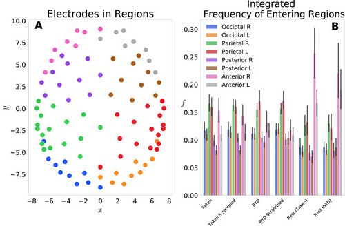
Abbildung 1: (A) Elektrodenpositionen für jede der 92 Elektroden auf der Kopfkappe von Electrical Geodesics Inc. Elektroden wurden auf eine horizontale Ebene mit der Nase in positiver y-Richtung projiziert. Die Elektroden wurden farbcodiert, um die Bestandteile der 8 Gruppen für die Frequenzanalyse anzuzeigen, nämlich okzipital links (blau)/rechts (orange), parietal links (grün)/rechts (rot), posterior links (lila)/ rechts (braun) und anterior links (rosa)/rechts (grau).
(B) Histogramme, die die Häufigkeit des Betretens jeder Region fG darstellen, werden für die sechs getesteten Bedingungen angezeigt. Beim Vergleich der Ruhe vor dem Stimulus und der jeweiligen stimulierten Bedingung ist eine signifikante Änderung innerhalb des Stimulus zwischen jeder der vorderen linken und rechten Regionen vorhanden (P < 0,001, Tukey-korrigiert.). Fehlerbalken zeigen das 1-Standardabweichungs-Konfidenzintervall an.
Phasenraum
Wir haben auch den mittelwertigen Phasenraum dieses Systems untersucht. Der Phasenraum für jedes Subjekt wurde als durchschnittliche Position und Impuls entlang der aufgetragen  Richtungoder als durchschnittliche Position und Impuls entlang der Richtung
 . Abbildung 2 zeigt die Schwerpunkte der Phasenraum-Streudiagramme für jedes Subjekt mit einer Ellipse, die das Konfidenzintervall einer Standardabweichung darstellt. Beachten Sie, dass Werte nur für die intakten Stimuli angegeben werden, da eine Varianzanalyse zeigt, dass die verschlüsselten und intakten Filme im Phasenraum nicht zu unterscheiden sind (
 , Tukey angepasst). Abbildung 2A und B zeigen die Projektion des Phasenraumschwerpunktes auf die aufgespannte Ebene Und
  für „Pang! You’re Dead“ bzw. „Taken“ und Abb. 2C und D (
 ) Ebene. Die durchschnittliche Position entlang der Achse
  denn der intakte Stimulus („BYD“ und „Taken“) und ihre verschlüsselten Formen unterscheiden sich signifikant von den Gegenstücken mit Ruhe vor dem Stimulus (Tukey angepasst), während die aufgabenpositiven und ruhenden Schwerpunkte in der nicht unterscheidbar sind Ebene (
 , Tukey angepasst). Die Mittelwerte der Gruppe sind in Tabelle 11 zusammen mit ihren Standardabweichungen angegeben. Diese Werte sind der gemittelte Wert der Schwerpunkte (Mittelwert der innerhalb der Stimulus-Mittelpunkte in Abb. 2) für die jeweilige Position/Impulse innerhalb jeder Stimulus-Ebene. Wie auch in Fig. 2C und D zu sehen ist, gibt es einen bemerkenswerten Unterschied von einer Größenordnung für
 zwischen den Ruhe- und Aufgabenbedingungen, jedoch keine deutlichen Unterschiede in ,
  order
order 
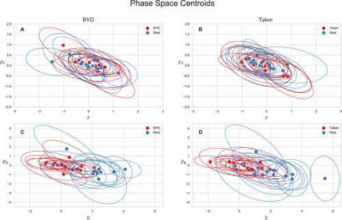
Abbildung 2: Mittlere Phasenraumschwerpunkte für jedes Subjekt. Ellipsen repräsentieren das 1-Standardabweichungs-Konfidenzintervall. Zentroide für die verschlüsselten Stimuli wurden weggelassen, da sie von intakten Stimuli nicht zu unterscheiden sind (P > 0,85) (A) Zentroide für „Bang! Du bist tot“ entlang der x-Richtung. (B) Schwerpunkte für „genommen“ entlang der x-Richtung. (C) Schwerpunkte für „Bang! Du bist tot“ entlang der y-Richtung. (D) Schwerpunkte für „genommen“ entlang der y-Richtung. Unterschiede sind nur in der y-Richtung erkennbar (P < 0,001, Tukey-korrigiert), was auf das höhere Maß an anteriorer Aktivierung hinweist, wie in Abb. 1 angegeben. Tabelle 1
Gruppenmittelwerte der Schwerpunkte.
| Stimulus
|

|
|
|
|
| Vergriffen
|

|

|

|

|
| Rührei genommen
|

|

|

|

|
| Knall! Du bist tot
|

|

|

|

|
| Knall! Du bist tot verschlüsselt
|

|

|

|

|
| Ruhe (vorher genommen)
|

|

|

|

|
| Ruhe (vor BYD)
|

|

|

|

|
Signifikante Unterschiede werden nur für den Rest festgestellt, der vor Taken and Bang erworben wurde! Sie sind tot, wenn Sie die durchschnittliche y-Position mit einem ihrer Aufgabengegenstücke vergleichen (verschlüsselter und intakter Stimulus).
Gruppenmittelwerte der Schwerpunkte.
Diese Analyse ergab zwei bemerkenswerte Ergebnisse. Erstens fehlten signifikante Unterschiede in den Impulsen des Gehirns entlang der x- und y-Richtung. Zweitens unterschieden sich die Durchschnitte in Momenta auf Gruppenebene nicht signifikant von 0. Die positiven oder negativen Impulse kommen von der konkurrierenden zeitlichen Ableitung der Wahrscheinlichkeit und des Ortes der Elektrode. Da die Impulse durchschnittlich 0 betragen, gibt es eine gleiche Anzahl anteriorer und posteriorer Elektroden mit sowohl Zunahmen als auch Abnahmen in der Wahrscheinlichkeit.
Außerdem untersuchten wir Änderungen der Wahrscheinlichkeitswerte sowohl im Ruhezustand als auch im aktiven Zustand. Animationen der Wahrscheinlichkeitsverteilungen sind in Ergänzungsmaterial 1 enthalten. In diesen Animationen werden die Unterschiede in Ruhe und Aufgabe durch die zeitliche Entwicklung der Wahrscheinlichkeit deutlich.
Unschärferelation
Trotz der Bestätigung früherer neurowissenschaftlicher Ergebnisse und des offensichtlichen Erfolgs unseres Quasi-Quantenmodells bleibt unsere oben gestellte Forschungsfrage nur halb beantwortet. Unter Verwendung dieses Modells stellten wir Unterschiede in den Wahrscheinlichkeitsverteilungen und den Phasenraumschwerpunkten in Ruhe im Vergleich zur Aufgabe fest. Wir suchten aber dennoch einen Parameter aus dem Modell, der in Ruhe und Aufgabe gleich bleibt. Dazu haben wir eine analoge Heisenbergsche Unschärferelation der Form
|
|

|

|
Tabelle 2 zeigt die Werte dieser Konstante () unter allen Bedingungen erfasst, sowie der Maximalwert, der Mittelwert und die Standardabweichung. Wir haben festgestellt, dass dieses Quasi-Quantenmodell zu einem konstanten Minimalwert über führt Und
Und  von
von  mit
mit  . Beachten Sie die Einheit von
 ist ein Ergebnis davon, dass das EEG bei 250 Hz abgetastet wird und die Masse als Einheit angenommen wird. Darüber hinaus bleiben der Durchschnittswert und die Standardabweichung dieser Größen über die Bedingungen hinweg konsistent mit einem Durchschnittswert von
  () und einer Standardabweichung von
  ( ). Bemerkenswerterweise variiert der Maximalwert zwischen den Bedingungen, wobei der größte Wert auftritt, während die Probanden den intakten Clip von Bang! Du bist tot. Obwohl die durchschnittliche Position des Signals entlang der y-Richtung in Ruhe anders ist als während einer Aufgabe () führt die quasi-quantenmathematische Methodik zu einem konstanten Unsicherheitswert. Bemerkenswerterweise zeigen die Werte in der Tabelle, dass die durchschnittliche Unsicherheit und die minimale Unsicherheit unter verschiedenen Bedingungen gleich sind, obwohl die Maxima um mehr als zwei Größenordnungen variieren. Dies verleiht der Idee, dass diese Unsicherheitsrelation die Ähnlichkeiten des Gehirns über die sehr unterschiedlichen Bedingungen hinweg erfasst, weitere Glaubwürdigkeit. Abbildung 3 zeigt die Wahrscheinlichkeitsverteilung zu dem Zeitpunkt, der dem Unsicherheitsminimum für und entspricht
Tabelle 2
Verschiedene Werte, die aus den Zeitverläufen der Produkte extrahiert wurden
and .
| Stimulus
|

|

|
|
|
|
|
|
|
| Vergriffen
|

|

|

|

|

|
|

|

|
| Rührei genommen
|

|

|

|

|

|

|
|

|
| Knall! Du bist tot
|

|

|

|

|

|

|

|

|
| Knall! Du bist tot verschlüsselt
|

|

|

|

|

|

|

|

|
| Ruhe (vorher genommen)
|

|

|

|

|

|
|
|

|
| Ruhe (vor BYD)
|

|

|

|

|

|

|

|

|
Betrachtet man den Mindestwert, den diese Produkte für jedes Fach erreichen, sehen wir einen konstanten Wert in x und y von, einen Durchschnittswert von und eine konstante Standardabweichung von . Die Einheit von ergibt sich aus der Abtastung von 250 Hz. Maximalwerte unterscheiden sich je nach Stimulation. Die Werte werden als Mittelwert über die Probanden plus oder minus 1 Standardabweichung angegeben.
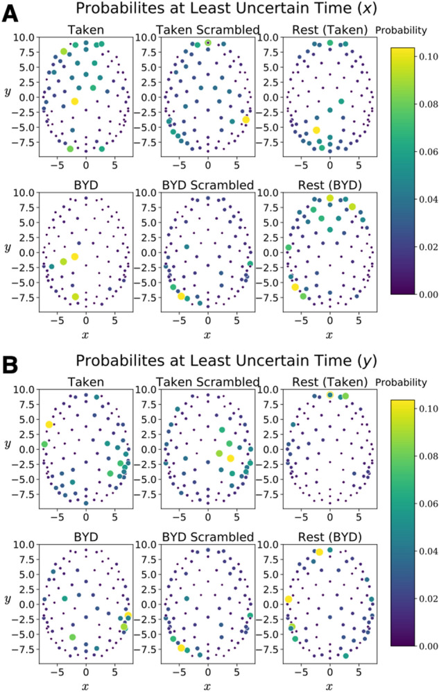
Abbildung 3: Wahrscheinlichkeitskarten, die dem am wenigsten unsicheren Zeitpunkt für jede der sechs experimentellen Bedingungen entsprechen. (A) Die Wahrscheinlichkeiten, die zu der minimalen Unsicherheit führen, definiert durch das Minimum von . (B) Die Wahrscheinlichkeiten, die zu der minimalen Unsicherheit führen, definiert durch das Minimum von . Ein Thema wird für alle Taken-Stimuli angezeigt und ein anderes für alle Bang! Du bist tot Reize. Diskussion
In der aktuellen Studie untersuchten wir das räumliche Ausmaß und die damit verbundenen Übergangseigenschaften der neuronalen Aktivität im Gehirn unter aktiven und Ruhebedingungen und ob ähnliche zugrunde liegende Netzwerkeigenschaften existieren. Wir fanden heraus, dass die Anwendung der Hilbert-Transformation auf die EEG-Daten und deren Normalisierung (Gleichung 2) dem EEG-Signal über das Gehirn (Gleichung 3) eine probabilistische Struktur auferlegt, die wir verwendeten, um die Wahrscheinlichkeit von räumlichen Aktivitätsmustern zusammen mit Übergängen zu identifizieren in Aktivität über die Kopfhaut. Wir fanden mehr anteriore Aktivität während der Ruhe im Vergleich zum Anschauen von Filmen, sowohl im Amplituden- als auch im Phasenraum. Dieser Befund steht im Einklang mit früheren Ergebnissen, die eine erhöhte Aktivierung im vorderen Bereich während der Ruhe zeigten.[21][21][22][34][37][38] Darüber hinaus konnten wir durch Normalisierung der Hilbert-transformierten EEG-Signale und Extrahieren von Durchschnittswerten, die denen der Wellenfunktionsformulierung der Quantenmechanik ähneln, die Unsicherheit in der „Position“ und dem „Impuls“ während der Ruhezeit und beim Ansehen von Filmen berechnen, die durch eingestellt werden die neue Konstante
 .
.
Es ist verlockend, die Konstante, die sich auf die „Position“ und den „Impuls“ der neuronalen Aktivität bezieht, mit einem fundamentalen Prinzip wie dem Heisenbergschen Unbestimmtheitsprinzip in Verbindung zu bringen. Was diese Ungewissheit bedeutet, ist jedoch noch unklar. Es könnte Grenzen für den Grad der Zugänglichkeit des Gehirns bedeuten; Zunehmende Informationen über den genauen Ort des Gehirnzustands (wie durch unsere Quasi-Quanten-„Wellenfunktionen“ beschrieben) werden eine größere Unsicherheit darüber erzeugen, wo er sich zu einem späteren Zeitpunkt befinden wird. Diese Ergebnisse bieten eine interessante Perspektive auf die Verbindung zwischen neuronaler Funktion und kognitiven Prozessen. Wenn zum Beispiel die „Wellenfunktion“ entlang eines Gedankengangs im Raum lokalisiert wird, werden wir abgelenkt, um die Unsicherheit zu erhöhen, was erklären könnte, warum Gedanken wandern und Gedanken flüchtig sind?
Ist der  Wert, den wir über verschiedene Stimulusbedingungen konstant fanden, und unabhängig von der Anzahl der Elektroden, die zum Erfassen der Daten verwendet wurden? Um dies zu testen, haben wir die EEG-Elektroden von 92 auf 20 abgetastet und die gleiche Analyse wie im Haupttext durchgeführt. In Übereinstimmung mit 92 Kanälen fanden wir die anteriore Tendenz in Ruhe, aber wir stellten fest, dass die Verringerung der Elektroden auf 20 zu einer anderen Konstante führte
  (Siehe Zusatzmaterial). Dies zeigt, dass das Modell in der Lage ist, die Unterschiede zwischen Ruhe und Aufgabe zu erfassen, aber möglicherweise muss eine montageabhängige Normalisierungsbedingung eingeführt werden.
Es ist wichtig zu beachten, dass Unsicherheitswerte dieser Form allen konjugierten Fourier-Variablen inhärent sind, da sich ein Wert in einer Variablen ausbreitet und in der anderen lokalisiert. Dies legt nahe, dass nach dem Definieren des Quadrats des zeitlichen Verlaufs der Hilbert-transformierten EEG-Elektrode als Wahrscheinlichkeit und dem Auferlegen der Eigenschaften eines Hilbert-Raums auf die Elektrodensignale ein Unsicherheitswert extrahiert werden kann. In der Quantenmechanik setzt diese Unsicherheit die Grenze für die nicht beobachtbaren Skalen. Dieser Ansatz wurde von der Notwendigkeit in der Neurowissenschaft nach neuartigen Modellen inspiriert, um bei der Interpretation von Neuroimaging-Daten zu helfen. Obwohl dies ein interessanter methodischer Fortschritt ist, müssen wir noch feststellen, ob die beobachtete Unsicherheit in den EEG-Daten durch ein neues Grundprinzip wie in der Quantenmechanik gestützt wird oder ob sie nur das Ergebnis der Bildung von zwei neuen konjugierten Fourier-Variablen aus der ist EEG-Signal.
Weitere Arbeiten müssen unternommen werden, um diese Konstante im Hinblick auf die reichhaltige Taxonomie von Aufgaben und Stimuli und unterschiedlichen Bewusstseinszuständen, die routinemäßig in der kognitiven Neurowissenschaft verwendet werden, zu erforschen. Diese Methodik könnte auf fMRI ausgedehnt werden, wo die BOLD-Zeitverläufe Hilbert-transformiert werden könnten, wodurch ein dreidimensionales Analogon des in diesem Artikel vorgestellten EEG-Modells entsteht.
Letztendlich stellte dieses Papier eine neuartige Methodik zur Analyse von EEG-Daten vor. Die Normalisierung der Daten und ihre Behandlung als Wahrscheinlichkeitsamplitude führte zu Parametern, die sich mit dem Vorhandensein oder Fehlen eines Stimulus änderten, während gleichzeitig ein konstanter Wert unabhängig vom Stimulus festgelegt wurde. Wir haben erfolgreich einen mathematischen Rahmen basierend auf den Formalismen der Quantenmechanik auf das Ruhe- und Aufgabenparadigma im EEG angewendet (ohne zu behaupten, dass das Gehirn ein Quantenobjekt ist). Da sich die Neurowissenschaften weiterentwickeln, müssen auch die ihr zur Verfügung stehenden Analysewerkzeuge entsprechend weiterentwickelt werden. Wir hoffen, dass dieses analytische Werkzeug zusammen mit den Fortschritten in der Modellierung und im maschinellen Lernen unser Verständnis der Natur des Bewusstseins unterstützen wird.
Methoden
Datenerfassung
28 gesunde Probanden wurden vom Brain and Mind Institute der University of Western Ontario, Kanada, rekrutiert, um an dieser Studie teilzunehmen. Vor dem Testen wurde von allen Teilnehmern eine schriftliche Zustimmung nach Aufklärung eingeholt. Die ethische Genehmigung für diese Studie wurde vom Health Sciences Research Ethics Board und dem Non-Medical Research Ethics Board der University of Western Ontario erteilt und die gesamte Forschung wurde in Übereinstimmung mit den relevanten Richtlinien/Vorschriften und in Übereinstimmung mit der Deklaration von Helsinki durchgeführt.
Als naturalistische Stimuli wurden in dieser Studie zwei spannende Filmclips verwendet. Ein Videoclip aus dem Stummfilm „Bang! Du bist tot“ und ein Audioausschnitt aus dem Film „Taken“ wurden 13 bzw. 15 Probanden sowohl in ihrer ursprünglichen intakten als auch verschlüsselten Form gezeigt. Vor den beiden Akquisitionen wurde ein Ruheabschnitt erworben, in dem die Probanden gebeten wurden, sich ohne offensichtliche Stimulation zu entspannen. Die Stimulus-Präsentation wurde mit dem Psychtoolbox-Plugin für MATLAB [39][40][41] auf einem 15″ Apple MacBook Pro gesteuert. Audio wurde binaural mit einer angenehmen Hörlautstärke über Etymotics ER-1-Kopfhörer präsentiert.
EEG-Daten wurden unter Verwendung einer 129-Kanal-Kappe (Electrical Geodesics Inc. [EGI], Oregon, USA) gesammelt. Die Elektrodenimpedanzen wurden unter 50 kΩ gehalten, wobei die Signale bei 250 Hz abgetastet und auf den zentralen Scheitelpunkt (Cz) bezogen wurden. Unter Verwendung der EEGLAB MATLAB-Toolbox wurden [42] verrauschte Kanäle identifiziert und entfernt und dann wieder in die Daten interpoliert. Ein Kolmogorov-Smirnov (KS)-Test an den Daten wurde verwendet, um Regionen zu identifizieren, die nicht gaußförmig waren. Eine unabhängige Komponentenanalyse (ICA) wurde dann verwendet, um Muster neuraler Aktivität, die für Augen- und Muskelbewegungen charakteristisch sind, visuell zu identifizieren, die anschließend aus den Daten entfernt wurden. Die EEG-Vorverarbeitung wurde individuell für jedes Subjekt und jeden Zustand durchgeführt.
Von den beiden getesteten Filmclips war der erste ein 8-minütiger Ausschnitt aus Alfred Hitchcocks TV-Stummfilm „Bang! Du bist tot". Diese Szene zeigt einen 5-jährigen Jungen, der den Revolver seines Onkels aufhebt. Der Junge lädt eine Kugel in die Waffe und spielt damit wie mit einem Spielzeug. Der Junge (und Betrachter) weiß selten, ob die Waffe eine Kugel in ihrer Kammer hat, und die Spannung baut sich auf, wenn der Junge die Kammer dreht, sie auf andere richtet und den Abzug drückt. Als Alternative zur visuellen Stimulation wurde auch ein 5-minütiger Audioausschnitt aus dem Film „Taken“ verwendet. Dieser Clip zeigt ein Telefongespräch, in dem ein Vater die Entführung seiner Töchter belauscht.
Außerdem wurden zwei „verwürfelte“ Kontrollreize verwendet – einer für jeden Film. Dies trennt die neuronalen Reaktionen, die durch die sensorischen Eigenschaften beim Ansehen oder Anhören der Filme ausgelöst werden, von denen, die an der Verfolgung der Handlung beteiligt sind. Die verschlüsselte Version von „Bang! Du bist tot“ wurde generiert, indem 1-Sekunden-Segmente isoliert und die Segmente pseudozufällig gemischt wurden, wodurch die zeitliche Kohärenz der Erzählung aufgehoben wurde. [43] Die verschlüsselte Version von „Taken“ wurde durch spektrale Rotation des Tons erstellt, wodurch die Sprache nicht entzifferbar wurde. [43][44] Die verschlüsselten Filmclips wurden vor den intakten Versionen präsentiert, um mögliche Übertragungseffekte der Erzählung zu vermeiden. Bevor die Versuchspersonen den verschlüsselten Stimulus beobachteten/hörten, wurde ein kurzes Segment des Ruhe-EEG erfasst.
Modell
Jede der j Elektroden wird durch ein geordnetes Paar beschrieben ( ) im dreidimensionalen Raum. Um diese Analyse abzuschließen, wurden die Elektroden zunächst auf die (
 ) Ebene, wobei die Tiefe des Kopfes entfernt wird. Fig. 1A zeigt die Positionen jeder Elektrode in diesem 2D-Raum. Nach dieser Projektion wurden die Zeitverläufe für jede der 92 Elektroden Hilbert-transformiert und dann gemäß dem unter Verwendung von Gl. (2). In diesem Elektrodenpositionsraum wurde eine Wahrscheinlichkeit als Quadrat des Hilbert-transformierten Zeitverlaufs definiert (Gl. 3), analog zu den Wellenfunktionen der Quantenmechanik. Acht Regionen Anterior L/R, Posterior L/R, Parietal L/R, Occipital L/R) wurden dann durch Gruppieren der 92 Elektroden definiert, und die Eintrittshäufigkeiten in jede Region fG wurden durch Summieren der Wahrscheinlichkeitselektroden innerhalb der Gruppe erhalten. dann rechtzeitig integrieren.
|
|

|

|
wobei jede der acht mit dem Index bezeichneten Gruppen eine unterschiedliche Anzahl von konstituierenden Elektroden N hat. Hinter dem Hinterkopf links und rechts sind jeweils 10 Elektroden, im Scheitelbereich links und rechts sind jeweils 17 Elektroden, im Hinterkopf links und rechts dort sind 10 bzw. 11 Elektroden, und vorne links und rechts befinden sich 8 bzw. 9 Elektroden.
Nach Erhalt der Frequenzen auf Gruppenebene wurden Mittelwerte für Position und Impuls unter Verwendung von Gl. (4) und (5) (mit identischen Ausdrücken für y). Schließlich suchten wir zur Feststellung unserer analogen Unbestimmtheitsrelation Ausdrücke der Form
|
|

|

|
Der Ausdruck for kann leicht auf die oben definierten Wahrscheinlichkeiten und Positionen angewendet werden, was zu dem ersten Term führt, der durch gegeben ist
|
|

|

|
Und der zweite Term, der durch das Quadrat von Gl. (4). Die zweite Amtszeit von  ist durch das Quadrat von Gl. (5), aber der erste Term ist nuancierter. Dies liegt an der komplexen Zahl, die zurückgegeben wird, wenn der Ableitungsoperator zweimal auf die Wahrscheinlichkeit angewendet wird. Um dies zu überwinden, wurden Fourier-Transformationen verwendet, um Gl. (5) in die Impulsbasis, die dann die effiziente Berechnung von ermöglichte
  .
.
Bezeichnung  als Impuls-Raum-Wahrscheinlichkeit, erhalten durch eine zweidimensionale, nicht gleichförmige Fourier-Transformation der Ortsraum-Pseudowellenfunktion, Gl. (5) kann umgeschrieben werden als
|
|

|

|
Führend zum ersten Term im zu schreibenden Ausdruck als,
|
|
![{\displaystyle \langle p_{x}^{2}(t)\rangle =m^{2}\sum _{j=1}^{92}{\tfrac {x_{j}^{2}}{{\tilde {p}}_{j}(t)}}[{d \over dt}P_{j}(t)]^{2}}](https://wikimedia.org/api/rest_v1/media/math/render/svg/3dda471e5a09b53812126091bf6b9a73fc19a4f4)
|

|
Der FINUFFT-Python-Wrapper wurde verwendet, um die Fourier-Transformation unter Verwendung einer ungleichmäßigen 2d-FFT[45][46] des Typs 3, 2d durchzuführen, und der zeitliche Minimalwert der Unsicherheitsrelation wurde gefunden. Punkte im Impulsraum wurden abgetastet ![{\displaystyle p_{x}\in [-4,4]}](https://wikimedia.org/api/rest_v1/media/math/render/svg/515f4df54a0052df61a308afa0bb41739bf89ef0) Und
Und ![{\displaystyle p_{y}\in [-4,5]}](https://wikimedia.org/api/rest_v1/media/math/render/svg/950ccba52979e32d86080daf5a94cb3b5524feb6) zusammen mit den zwei zusätzlichen Punkten (
zusammen mit den zwei zusätzlichen Punkten (![{\displaystyle [-5,-4]}](https://wikimedia.org/api/rest_v1/media/math/render/svg/c1acb0cb7df6bce649ff45049f7f85ca28c1c5b7) ) Und (
) Und (![{\displaystyle [-4,-5]}](https://wikimedia.org/api/rest_v1/media/math/render/svg/c01ceeb13f42e4e0cc0444eefecc2e668333a503) )
)
Abbildung 4 zeigt die Orts- und Impulswahrscheinlichkeiten jeweils in ihrer eigenen Basis. Eine Animation, die zeigt, wie sich diese im Laufe der Zeit für die verschiedenen Bedingungen entwickeln, ist in Ergänzungsmaterial 2 dargestellt.
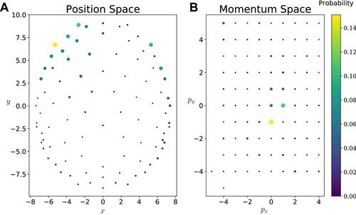
Abbildung 4: (A) Wahrscheinlichkeitsverteilung für ein einzelnes Subjekt in der Positionsbasis. (B) Momentum-Basis-Wahrscheinlichkeitsverteilung für ein einzelnes Subjekt. Die für die Fourier-Transformation verwendeten Impulswerte sind durch die Punktpositionen angegeben. Punkte sind farb-/größencodiert, um den Wahrscheinlichkeitswert an dieser Stelle darzustellen. Um die in Tabelle 2 angegebenen Werte zu berechnen, wurde für jedes Subjekt der entsprechende Wert gefunden, und diese wurden verwendet, um den hier angegebenen Gruppendurchschnitt zu berechnen.
Ergänzende Angaben
Ergänzende Zahlen.(28M, docx)
Ergänzende Informationen.(375K, docx)
Danksagungen
Wir möchten Silvano Petrarca für seine fortwährende Unterstützung bei der Entwicklung des Modells danken. Diese Studie wurde vom NSERC Discovery Grant (05578–2014RGPIN), CERC (215063), CIHR Foundation Fund (167264) finanziert. AMO ist Fellow des CIFAR Brain, Mind and Consciousness Program.
Autorenbeiträge
N.J.M.P., C.M. und G. L. führten die Analyse durch. A. S., B. S. und N.J.M.P. das Modell entwickelt. ALS. und B.S. überwachte die Analyse. N.J.M.P., A.S., G.L. und B.S. schrieb das Manuskript. A.M.O. überarbeitete das Manuskript.
Konkurrierende Interessen
Die Autoren erklären keine konkurrierenden Interessen.
Fußnoten
Anmerkung des Herausgebers
Springer Nature bleibt neutral in Bezug auf Zuständigkeitsansprüche in veröffentlichten Karten und institutionellen Zugehörigkeiten.
Diese Autoren haben zu gleichen Teilen beigetragen: Bobby Stojanoski und Andrea Soddu.
Ergänzende Angaben
Die Online-Version enthält ergänzendes Material, das unter 10.1038/s41598-021-97960-7 verfügbar ist.
Artikelinformationen
Sci Rep. 2021; 11: 19771.
Published online 2021 Oct 5. doi: 10.1038/s41598-021-97960-7
PMCID: PMC8492705
PMID: 34611185
Nicholas J. M. Popiel,1,2 Colin Metrow,1 Geoffrey Laforge,3 Adrian M. Owen,3,4,5 Bobby Stojanoski,#4,6 and Andrea Soddu#1,3
1The Department of Physics and Astronomy, The University of Western Ontario, London, ON N6A 5B7 Canada
2Cavendish Laboratory, University of Cambridge, Cambridge, CB3 0HE UK
3The Brain and Mind Institute, The University of Western Ontario, London, ON N6A 5B7 Canada
4The Department of Psychology, The University of Western Ontario, London, ON N6A 5B7 Canada
5The Department of Physiology and Pharmacology, The University of Western Ontario, London, ON N6A 5B7 Canada
6Faculty of Social Science and Humanities, University of Ontario Institute of Technology, 2000 Simcoe Street North, Oshawa, ON L1H 7K4 Canada
Andrea Soddu, Email: asoddu@uwo.ca
Corresponding author.
- Contributed equally.
Received 2021 Apr 28; Accepted 2021 Aug 30.
Copyright © The Author(s) 2021
Offener Zugang
Dieser Artikel ist unter einer Creative Commons Attribution 4.0 International License lizenziert, die die Verwendung, gemeinsame Nutzung, Anpassung, Verbreitung und Reproduktion in jedem Medium oder Format erlaubt, solange Sie den ursprünglichen Autor (die ursprünglichen Autoren) und die Quelle angemessen erwähnen, a Link zur Creative-Commons-Lizenz und geben Sie an, ob Änderungen vorgenommen wurden. Die Bilder oder andere Materialien von Drittanbietern in diesem Artikel sind in der Creative Commons-Lizenz des Artikels enthalten, sofern in einer Quellenangabe für das Material nichts anderes angegeben ist. Wenn Material nicht in der Creative-Commons-Lizenz des Artikels enthalten ist und Ihre beabsichtigte Nutzung durch gesetzliche Bestimmungen nicht gestattet ist oder die zulässige Nutzung überschreitet, müssen Sie die Genehmigung direkt vom Urheberrechtsinhaber einholen. Um eine Kopie dieser Lizenz anzuzeigen, besuchen
Sie http://creativecommons.org/licenses/by/4.0/.
Artikel aus wissenschaftlichen Berichten werden hier mit freundlicher Genehmigung von == Nature Publishing Group == zur Verfügung gestellt
Bibliography & references
- ↑ Biswal B, Zerrin Yetkin F, Haughton VM, Hyde JS, «Functional connectivity in the motor cortex of resting human brain using echo-planar MRI», in Magn Reson Med, 1995».
PMID:8524021
DOI:10.1002/mrm.1910340409
- ↑ Hutchison RM, Womelsdorfb T, Allenc EA, Bandettini PA, Calhound VD, Corbetta M, Della Penna S, «Dynamic functional connectivity: Promise, issues, and interpretations», in Neuroimage, 2013».
PMID:23707587 - PMCID:PMC3807588
DOI:10.1016/j.neuroimage.2013.05.079
- ↑ Eickhoff SB, Yeo BTT, Genon S, «Imaging-based parcellations of the human brain», in Nat Rev Neurosci, 2018».
PMID:30305712
DOI:10.1038/s41583-018-0071-7
- ↑ Dajani DR, Burrows CA, Odriozola P, Baez A, Nebel MB, Mostofsky SH, Uddin LQ, «Investigating functional brain network integrity using a traditional and novel categorical scheme for neurodevelopmental disorders», in NeuroImage Clin, 2019».
PMID:30708240 - PMCID:PMC6356009
DOI:10.1016/j.nicl.2019.101678
- ↑ Uddin LQ, Karlsgodt KH, «Future directions for examination of brain networks in neurodevelopmental disorders», in J Clin Child Adolesc Psychol, Society of Clinical Child & Adolescent Psychology, 2018».
PMID:29634380 - PMCID:PMC6842321
DOI:10.1080/15374416.2018.1443461
- ↑ Sripada C, Rutherford S, Angstadt M, Thompson WK, Luciana M, Weigard A, Hyde LH, «Prediction of neurocognition in youth from resting state fMRI», in Mol Psychiatry, 2020».
PMID:31427753 - PMCID:PMC7055722
DOI:10.1038/s41380-019-0481-6
- ↑ Biswal BB, Eldreth DA, Motes MA, Rypma B. Task-dependent individual differences in prefrontal connectivity. Cereb. Cortex. 2010;20:2188–2197. doi: 10.1093/cercor/bhp284. [PMC free article][PubMed] [CrossRef] [Google Scholar]
- ↑ Fox MD, Raichle ME. Spontaneous fluctuations in brain activity observed with functional magnetic resonance imaging. Nat. Rev. Neurosci. 2007;8:700–711. doi: 10.1038/nrn2201. [PubMed] [CrossRef] [Google Scholar]
- ↑ Kraus BT, et al. Network variants are similar between task and rest states. Neuroimage. 2021;229:117743. doi: 10.1016/j.neuroimage.2021.117743. [PMC free article][PubMed] [CrossRef] [Google Scholar]
- ↑ Kristo G, et al. Task and task-free FMRI reproducibility comparison for motor network identification. Hum. Brain Mapp. 2014;35:340–352. doi: 10.1002/hbm.22180. [PMC free article][PubMed] [CrossRef] [Google Scholar]
- ↑ Sui J, Adali T, Pearlson GD, Calhoun VD. An ICA-based method for the identification of optimal FMRI features and components using combined group-discriminative techniques. Neuroimage. 2009;46:73–86. doi: 10.1016/j.neuroimage.2009.01.026.[PMC free article] [PubMed] [CrossRef] [Google Scholar]
- ↑ Calhoun VD, Kiehl KA, Pearlson GD. Modulation of temporally coherent brain networks estimated using ICA at rest and during cognitive tasks. Hum. Brain Mapp. 2008;29:828–838. doi: 10.1002/hbm.20581. [PMC free article] [PubMed] [CrossRef] [Google Scholar]
- ↑ Xie H, et al. Whole-brain connectivity dynamics reflect both task-specific and individual-specific modulation: A multitask study. Neuroimage. 2018;180:495–504. doi: 10.1016/j.neuroimage.2017.05.050. [PMC free article] [PubMed] [CrossRef] [Google Scholar]
- ↑ Naci L, Cusack R, Anello M, Owen AM. A common neural code for similar conscious experiences in different individuals. Proc. Natl. Acad. Sci. U. S. A. 2014;111:14277–14282. doi: 10.1073/pnas.1407007111. [PMC free article] [PubMed] [CrossRef] [Google Scholar]
- ↑ Kannurpatti SS, Rypma B, Biswal BB. Prediction of task-related BOLD fMRI with amplitude signatures of resting-state fMRI. Front. Syst. Neurosci. 2012;6:7. doi: 10.3389/fnsys.2012.00007.[PMC free article] [PubMed] [CrossRef] [Google Scholar]
- ↑ Elliott ML, et al. General functional connectivity: Shared features of resting-state and task fMRI drive reliable and heritable individual differences in functional brain networks. Neuroimage. 2019;189:516–532. doi: 10.1016/j.neuroimage.2019.01.068. [PMC free article][PubMed] [CrossRef] [Google Scholar]
- ↑ Cole MW, Ito T, Cocuzza C, Sanchez-Romero R. The functional relevance of task-state functional connectivity. J. Neurosci. 2021 doi: 10.1523/JNEUROSCI.1713-20.2021. [PMC free article][PubMed] [CrossRef] [Google Scholar]
- ↑ Zhang S, et al. Characterizing and differentiating task-based and resting state fMRI signals via two-stage sparse representations. Brain Imaging Behav. 2016;10:21–32. doi: 10.1007/s11682-015-9359-7.[PMC free article] [PubMed] [CrossRef] [Google Scholar]
- ↑ Monier C, Chavane F, Baudot P, Graham LJ, Frégnac Y. Orientation and direction selectivity of synaptic inputs in visual cortical neurons: A diversity of combinations produces spike tuning. Neuron. 2003;37:663–680. doi: 10.1016/S0896-6273(03)00064-3.[PubMed] [CrossRef] [Google Scholar]
- ↑ Churchland MM, et al. Stimulus onset quenches neural variability: A widespread cortical phenomenon. Nat. Neurosci. 2010;13:369–378. doi: 10.1038/nn.2501. [PMC free article][PubMed] [CrossRef] [Google Scholar]
- ↑ 21.0 21.1 21.2 He BJ. Spontaneous and task-evoked brain activity negatively interact. J. Neurosci. 2013;33:4672–4682. doi: 10.1523/JNEUROSCI.2922-12.2013. [PMC free article][PubMed] [CrossRef] [Google Scholar]
- ↑ 22.0 22.1 22.2 Bonnard M, et al. Resting state brain dynamics and its transients: A combined TMS-EEG study. Sci. Rep. 2016;6:1–9. doi: 10.1038/srep31220. [PMC free article] [PubMed] [CrossRef] [Google Scholar]
- ↑ 23.0 23.1 Axelrod V, Zhu X, Qiu J. Transcranial stimulation of the frontal lobes increases propensity of mind-wandering without changing meta-awareness. Sci. Rep. 2018;8:1–14. doi: 10.1038/s41598-018-34098-z. [PMC free article] [PubMed] [CrossRef] [Google Scholar]
- ↑ 24.0 24.1 24.2 Axelrod V, Rees G, Lavidor M, Bar M. Increasing propensity to mind-wander with transcranial direct current stimulation. Proc. Natl. Acad. Sci. U. S. A. 2015;112:3314–3319. doi: 10.1073/pnas.1421435112. [PMC free article] [PubMed] [CrossRef] [Google Scholar]
- ↑ 25.0 25.1 Townsend JS. A Modern Approach to Quantum Mechanics.University Science Books; 2012. [Google Scholar]
- ↑ Heisenberg W. Über den anschaulichen Inhalt der quantentheoretischen Kinematik und Mechanik. Z. Phys. 1927;43:172–198. doi: 10.1007/BF01397280. [CrossRef] [Google Scholar]
- ↑ Penrose R. The Emperor’s New Mind. Viking Penguin; 1990. [Google Scholar]
- ↑ Penrose R. Shadows of the Mind: A Search for the Missing Science of Consciousness. Oxford University Press; 1994. [Google Scholar]
- ↑ Atmanspacher H. Quantum Approaches to Consciousness.Stanford Encyclopedia of Philosophy; 2004. [Google Scholar]
- ↑ Hameroff S. How quantum brain biology can rescue conscious free will. Front. Integr. Neurosci. 2012;6:93. doi: 10.3389/fnint.2012.00093. [PMC free article] [PubMed] [CrossRef] [Google Scholar]
- ↑ Freeman WJ, Vitiello G. Nonlinear brain dynamics as macroscopic manifestation of underlying many-body field dynamics. Phys. Life Rev. 2006;3:93–118. doi: 10.1016/j.plrev.2006.02.001.[CrossRef] [Google Scholar]
- ↑ le Van Quyen M, et al. Comparison of Hilbert transform and wavelet methods for the analysis of neuronal synchrony. J. Neurosci. Methods. 2001;111:83–98. doi: 10.1016/S0165-0270(01)00372-7.[PubMed] [CrossRef] [Google Scholar]
- ↑ Freeman WJ. Deep analysis of perception through dynamic structures that emerge in cortical activity from self-regulated noise. Cogn. Neurodyn. 2009;3:105–116. doi: 10.1007/s11571-009-9075-3.[PMC free article] [PubMed] [CrossRef] [Google Scholar]
- ↑ 34.0 34.1 Wang RWY, Chang WL, Chuang SW, Liu IN. Posterior cingulate cortex can be a regulatory modulator of the default mode network in task-negative state. Sci. Rep. 2019;9:1–12. [PMC free article][PubMed] [Google Scholar]
- ↑ Uddin LQ, Kelly AMC, Biswal BB, Castellanos FX, Milham MP. Functional connectivity of default mode network components: Correlation, anticorrelation, and causality. Hum. Brain Mapp. 2009;30:625–637. doi: 10.1002/hbm.20531. [PMC free article][PubMed] [CrossRef] [Google Scholar]
- ↑ Stawarczyk D, Majerus S, Maquet P, D’Argembeau A. Neural correlates of ongoing conscious experience: Both task-unrelatedness and stimulus-independence are related to default network activity. PLoS One. 2011;6:e16997. doi: 10.1371/journal.pone.0016997.[PMC free article] [PubMed] [CrossRef] [Google Scholar]
- ↑ 37.0 37.1 Greicius, M. D., Krasnow, B., Reiss, A. L., Menon, V. & Raichle, M. E. Functional Connectivity in the Resting Brain: A Network Analysis of the Default Mode Hypothesis. www.pnas.org. [PMC free article] [PubMed]
- ↑ Christoff K, Gordon AM, Smallwood J, Smith R, Schooler JW. Experience sampling during fMRI reveals default network and executive system contributions to mind wandering. Proc. Natl. Acad. Sci. U. S. A. 2009;106:8719–8724. doi: 10.1073/pnas.0900234106.[PMC free article] [PubMed] [CrossRef] [Google Scholar]
- ↑ Brainard DH. The psychophysics toolbox. Spat. Vis. 1997;10:433–436. doi: 10.1163/156856897X00357. [PubMed] [CrossRef] [Google Scholar]
- ↑ Kleiner M, et al. What’s new in psychtoolbox-3. Perception. 2007;36:1–16. [Google Scholar]
- ↑ Pelli DG. The VideoToolbox software for visual psychophysics: Transforming numbers into movies. Spat. Vis. 1997;10:437–442. doi: 10.1163/156856897X00366. [PubMed] [CrossRef] [Google Scholar]
- ↑ Makeig, S. & Onton, J. ERP features and EEG dynamics: An ICA perspective. In The Oxford Handbook of Event-Related Potential Components (Oxford University Press, 2012). 10.1093/oxfordhb/9780195374148.013.0035.
- ↑ 43.0 43.1 Laforge G, Gonzalez-Lara LE, Owen AM, Stojanoski B. Individualized assessment of residual cognition in patients with disorders of consciousness. NeuroImage Clin. 2020;28:102472. doi: 10.1016/j.nicl.2020.102472. [PMC free article] [PubMed] [CrossRef] [Google Scholar]
- ↑ Naci L, Sinai L, Owen AM. Detecting and interpreting conscious experiences in behaviorally non-responsive patients. Neuroimage. 2017;145:304–313. doi: 10.1016/j.neuroimage.2015.11.059.[PubMed] [CrossRef] [Google Scholar]
- ↑ Barnett AH, Magland J, Klinteberg LAF. A parallel nonuniform fast Fourier transform library based on an “Exponential of semicircle” kernel. SIAM J. Sci. Comput. 2019;41:C479–C504. doi: 10.1137/18M120885X. [CrossRef] [Google Scholar]
- ↑ Barnett, A. H. Aliasing error of the kernel in the nonuniform fast Fourier transform. arXiv:2001.09405 [math.NA] (2020).
Masticationpedia is a charity, a not-for-profit organization operating in dentistry medical research,
particularly focusing on the field of the neurophysiology of the masticatory system


